Section 14.8: Lagrange Multipliers
| Site: | Freebirds Moodle |
| Course: | Mathematical Methods I - SNIOE - Monsoon 2025 |
| Book: | Section 14.8: Lagrange Multipliers |
| Printed by: | Guest user |
| Date: | Monday, 9 February 2026, 8:11 AM |
Table of contents
- Section Learning outcomes
- Lagrange Multipliers Theory
- Method of Lagrange Multipliers
- Lagrange Multiplier - Example
- Example 2
- Example: Optimize a function over bounded domain
- Example: Optimize a function over bounded domain
- Two constraint - Lagrange Multipliers
- Example: Two constraint Lagrange Multipliers
- Exercise 1
- Exercise 2
- Exercise 3
- Exercise 4
- Exercise 5
- Exercise 6
- Exercise 7
- Exercise 8
- Exercise 9
- Exercise 10
- Exercise 11
- Exercise 12
- Exercise 13
- Exercise 14
- Exercise 15
- Exercise 16
- Exercise 17
- Exercise 18
- Exercise 19
- Exercise 20
- Exercise 21
- Exercise 22
- Exercise 23
- Exercise 24
- Exercise 25
- Exercise 26
- Exercise 27
- Exercise 28
- Exercise 29
- Exercise 30
- Exercise 31
- Exercise 32
- Exercise 33
- Exercise 34
- Exercise 35
- Exercise 36
- Exercise 37
- Exercise 38
- Exercise 39
- Exercise 40
- Exercise 41
- Exercise 42
- Exercise 43
- Exercise 44
- Exercise 45
- Exercise 46
- Exercise 47
- Exercise 48
- Exercise 49
- Exercise 50
Section Learning outcomes
- Use of Lagrange Multipliers to optimize a function over curves and surfaces
Lagrange Multipliers Theory
In a previous example, we maximized a volume function \(V = xyz\) subject to the constraint \(2xz + 2yz + xy = 12\), which expressed the side condition that the surface area was 12 m\(^2\).
In this section we present Lagrange’s method for maximizing or minimizing a general function \(f(x, y, z)\) subject to a constraint (or side condition) of the form \(g(x, y, z) = k\).
It’s easier to explain the geometric basis of Lagrange’s method for functions of two variables. So we start by trying to find the extreme values of \(f(x, y)\) subject to a constraint of the form \(g(x, y) = k\). In other words, we seek the extreme values of \(f(x, y)\) when the point \((x, y)\) is restricted to lie on the level curve \(g(x, y) = k\).
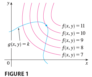
Figure 1 shows this curve together with several level curves of \(f\). These have the equations \(f(x, y) = c\), where \(c = 7, 8, 9, 10, 11\). To maximize \(f(x, y)\) subject to \(g(x, y) = k\) is to find the largest value of \(c\) such that the level curve \(f(x, y) = c\) intersects \(g(x, y) = k\). It appears from Figure 1 that this happens when these curves just touch each other, that is, when they have a common tangent line. (Otherwise, the value of \(c\) could be increased further.) This means that the normal lines at the point \((x_0, y_0)\) where they touch are identical. So the gradient vectors are parallel; that is, \(\nabla f(x_0, y_0) = \lambda \nabla g(x_0, y_0)\) for some scalar \(\lambda\).
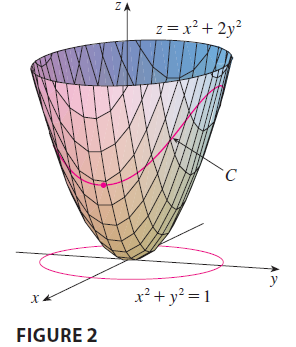
This kind of argument also applies to the problem of finding the extreme values of \(f(x, y, z)\) subject to the constraint \(g(x, y, z) = k\). Thus the point \((x, y, z)\) is restricted to lie on the level surface \(S\) with equation \(g(x, y, z) = k\). Instead of the level curves in Figure 1, we consider the level surfaces \(f(x, y, z) = c\) and argue that if the maximum value of \(f\) is \(f(x_0, y_0, z_0) = c\), then the level surface \(f(x, y, z) = c\) is tangent to the level surface \(g(x, y, z) = k\) and so the corresponding gradient vectors are parallel.
This intuitive argument can be made precise as follows. Suppose that a function \(f\) has an extreme value at a point \(P(x_0, y_0, z_0)\) on the surface \(S\) and let \(C\) be a curve with vector equation \(\mathbf{r}(t) = \langle x(t), y(t), z(t) \rangle\) that lies on \(S\) and passes through \(P\). If \(t_0\) is the parameter value corresponding to the point \(P\), then \(\mathbf{r}(t_0) = \langle x_0, y_0, z_0 \rangle\). The composite function \(h(t) = f(x(t), y(t), z(t))\) represents the values that \(f\) takes on the curve \(C\). Since \(f\) has an extreme value at \((x_0, y_0, z_0)\), it follows that \(h\) has an extreme value at \(t_0\), so \(h'(t_0) = 0\). But if \(f\) is differentiable, we can use the Chain Rule to write \[ 0 = h'(t_0) = f_x(x_0, y_0, z_0)x'(t_0) + f_y(x_0, y_0, z_0)y'(t_0) + f_z(x_0, y_0, z_0)z'(t_0) = \nabla f(x_0, y_0, z_0) \cdot \mathbf{r}'(t_0) \] This shows that the gradient vector \(\nabla f(x_0, y_0, z_0)\) is orthogonal to the tangent vector \(\mathbf{r}'(t_0)\) to every such curve \(C\). But we already know that the gradient vector of \(g\), \(\nabla g(x_0, y_0, z_0)\), is also orthogonal to \(\mathbf{r}'(t_0)\) for every such curve. This means that the gradient vectors \(\nabla f(x_0, y_0, z_0)\) and \(\nabla g(x_0, y_0, z_0)\) must be parallel. Therefore, if \(\nabla g(x_0, y_0, z_0) \neq \mathbf{0}\), there is a number \(\lambda\) such that \[ \nabla f(x_0, y_0, z_0) = \lambda \nabla g(x_0, y_0, z_0) \] The number \(\lambda\) in Equation 1 is called a Lagrange multiplier. The procedure is described the next page.
Method of Lagrange Multipliers
Method of Lagrange Multipliers To find the maximum and minimum values of \(f(x, y, z)\) subject to the constraint \(g(x, y, z) = k\) [assuming that these extreme values exist and \(\nabla g \neq \mathbf{0}\) on the surface \(g(x, y, z) = k\)]: (a) Find all values of \(x, y, z\), and \(\lambda\) such that \[ \nabla f(x, y, z) = \lambda \nabla g(x, y, z) \] and \[ g(x, y, z) = k \] (b) Evaluate \(f\) at all the points \((x, y, z)\) that result from step (a). The largest of these values is the maximum value of \(f\); the smallest is the minimum value of \(f\).
If we write the vector equation \(\nabla f = \lambda \nabla g\) in terms of components, then the equations in step (a) become \[ f_x = \lambda g_x \quad f_y = \lambda g_y \quad f_z = \lambda g_z \quad g(x, y, z) = k \] This is a system of four equations in the four unknowns \(x, y, z\), and \(\lambda\), but it is not necessary to find explicit values for \(\lambda\).
For functions of two variables the method of Lagrange multipliers is similar to the method just described. To find the extreme values of \(f(x, y)\) subject to the constraint \(g(x, y) = k\), we look for values of \(x, y\), and \(\lambda\) such that \[ \nabla f(x, y) = \lambda \nabla g(x, y) \quad \text{and} \quad g(x, y) = k \] This amounts to solving three equations in three unknowns: \[ f_x = \lambda g_x \quad f_y = \lambda g_y \quad g(x, y) = k \]
Lagrange Multiplier - Example
EXAMPLE 1 A rectangular box without a lid is to be made from 12 m\(^2\) of cardboard. Find the maximum volume of such a box.
Example 2
EXAMPLE 2 Find the extreme values of the function \(f(x, y) = x^2 + 2y^2\) on the circle \(x^2 + y^2 = 1\).
Example: Optimize a function over bounded domain
EXAMPLE 3 Find the extreme values of \(f(x, y) = x^2 + 2y^2\) on the disk \(x^2 + y^2 \le 1\).
Example: Optimize a function over bounded domain
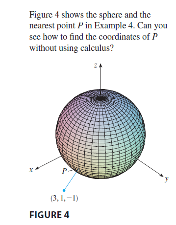
EXAMPLE 4 Find the points on the sphere \(x^2 + y^2 + z^2 = 4\) that are closest to and farthest from the point \((3, 1, -1)\).
Two constraint - Lagrange Multipliers
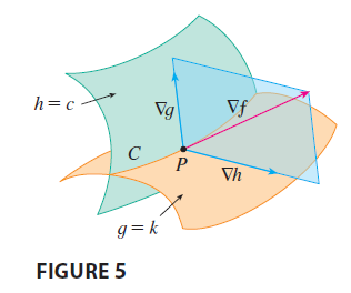
Suppose now that we want to find the maximum and minimum values of a function \(f(x, y, z)\) subject to two constraints (side conditions) of the form \(g(x, y, z) = k\) and \(h(x, y, z) = c\). Geometrically, this means that we are looking for the extreme values of \(f\) when \((x, y, z)\) is restricted to lie on the curve of intersection \(C\) of the level surfaces \(g(x, y, z) = k\) and \(h(x, y, z) = c\). Suppose \(f\) has such an extreme value at a point \(P(x_0, y_0, z_0)\). We know that \(\nabla f\) is orthogonal to \(C\) at \(P\). But we also know that \(\nabla g\) and \(\nabla h\) are orthogonal to \(C\) at \(P\). This means that the gradient vector \(\nabla f(x_0, y_0, z_0)\) is in the plane determined by \(\nabla g(x_0, y_0, z_0)\) and \(\nabla h(x_0, y_0, z_0)\). (We assume that these gradient vectors are not zero and not parallel.) So there are numbers \(\lambda\) and \(\mu\) (called Lagrange multipliers) such that \[ \nabla f(x_0, y_0, z_0) = \lambda \nabla g(x_0, y_0, z_0) + \mu \nabla h(x_0, y_0, z_0) \] In this case Lagrange’s method is to look for extreme values by solving five equations in the five unknowns \(x, y, z, \lambda,\) and \(\mu\). These equations are obtained by writing Equation 16 in terms of its components and using the constraint equations: \[ f_x = \lambda g_x + \mu h_x \] \[ f_y = \lambda g_y + \mu h_y \] \[ f_z = \lambda g_z + \mu h_z \] \[ g(x, y, z) = k \] \[ h(x, y, z) = c \]
Example: Two constraint Lagrange Multipliers
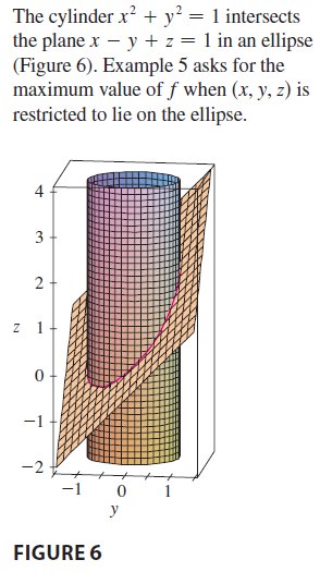
EXAMPLE 5 Find the maximum value of the function \(f(x, y, z) = x + 2y + 3z\) on the curve of intersection of the plane \(x - y + z = 1\) and the cylinder \(x^2 + y^2 = 1\).
 |
Exercise 1
Pictured are a contour map of \(f\)
and a curve with equation \(g(x, y) =
8\). Estimate the maximum and minimum values of \(f\) subject to the constraint that \(g(x, y) = 8\). Explain your reasoning. 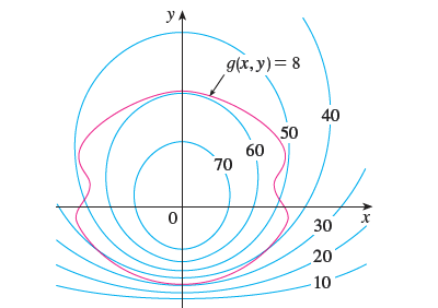
Exercise 2
- Use a graphing calculator or computer to graph the curve with equation \(x^3 + y^3 = 3xy\). At what point on the curve does it seem that the tangent line is horizontal?
- Use the method of Lagrange multipliers to find the exact coordinates of the point in part (a).
Exercise 3
Find the extreme values of \(f(x, y) = x^2 + y^2\) subject to the constraint \(xy = 1\).
Exercise 4
Find the extreme values of \(f(x, y) = xy\) subject to the constraint \(x^2 + y^2 = 1\).
Exercise 5
Find the extreme values of \(f(x, y) = x^2 + 2y^2\) subject to the constraint \(x^2 + y^2 = 1\).
Exercise 6
Find the extreme values of \(f(x, y) = x^2 - y^2\) subject to the constraint \(x^2 + y^2 = 1\).
Exercise 7
Find the extreme values of \(f(x, y, z) = 2x + 2y + z\) subject to the constraint \(x^2 + y^2 + z^2 = 9\).
Exercise 8
Find the extreme values of \(f(x, y, z) = x^2 + y^2 + z^2\) subject to the constraint \(x + y + z = 12\).
Exercise 9
Find the extreme values of \(f(x, y, z) = xyz\) subject to the constraint \(x^2 + 2y^2 + 3z^2 = 6\).
Exercise 10
Find the extreme values of \(f(x, y, z) = x^2y^2z^2\) subject to the constraint \(x^2 + y^2 + z^2 = 1\).
Exercise 11
Find the extreme values of \(f(x, y, z) = x^4 + y^4 + z^4\) subject to the constraint \(x^2 + y^2 + z^2 = 1\).
Exercise 12
Find the extreme values of \(f(x, y, z, t) = x + y + z + t\) subject to the constraint \(x^2 + y^2 + z^2 + t^2 = 1\).
Exercise 13
Find the extreme values of \(f(x_1, x_2, ..., x_n) = x_1 + x_2 + ... + x_n\) subject to the constraint \(x_1^2 + x_2^2 + ... + x_n^2 = 1\).
Exercise 14
Find the extreme values of \(f(x_1, x_2, ..., x_n) = x_1^2 + x_2^2 + ... + x_n^2\) subject to the constraint \(x_1 + x_2 + ... + x_n = 1\).
Exercise 15
The method of Lagrange multipliers assumes that the extreme values exist, but that is not always the case. Show that the problem of finding the minimum value of \(f(x, y) = x\) subject to the constraint \(y^2 + x^4 - x^3 = 0\) can be solved using Lagrange multipliers, but \(f\) does not have a maximum value with that constraint.
Exercise 16
Find the maximum value of \(f(x, y) = e^{xy}\) subject to the constraint \(x^3 + y^3 = 16\). Show that \(f\) has no minimum value with this constraint.
Exercise 17
Find the extreme values of \(f(x, y) = x^2 + y^2\) subject to both constraints \(x^2 + y^2 = 1\) and \(x + y = 1\).
Exercise 18
Find the extreme values of \(f(x, y, z) = x^2 + y^2 + z^2\) subject to both constraints \(x^2 + y^2 + z^2 = 1\) and \(x + y + z = 1\).
Exercise 19
Find the extreme values of \(f(x, y, z) = yz + xy\) subject to both constraints \(xy = 1\) and \(y^2 + z^2 = 1\).
Exercise 20
Find the extreme values of \(f(x, y, z) = x^2 + y^2 + z^2\) subject to both constraints \(z^2 = x^2 + y^2\) and \(x + y - z = -1\).
Exercise 21
Find the absolute maximum and minimum values of \(f(x, y) = x^2y\) on the ellipse \(x^2 + 2y^2 = 6\).
Exercise 22
Find the absolute maximum and minimum values of \(f(x, y) = x^2 + 4x + y^2 - 4y\) on the disk \(x^2 + y^2 \le 9\).
Exercise 23
Find the absolute maximum and minimum values of \(f(x, y) = 2x^2 + 3y^2 - 4x - 5\) on the disk \(x^2 + y^2 \le 16\).
Exercise 24
Find the absolute maximum and minimum values of \(f(x, y) = e^{-x^2-y^2}(x^2 + 2y^2)\) on the disk \(x^2 + y^2 \le 4\).
Exercise 25
Consider the problem of maximizing the function \(f(x, y) = 2x + 3y\) subject to the constraint \(\sqrt{x} + \sqrt{y} = 5\). (a) Try using Lagrange multipliers to solve the problem. (b) Does \(f(25, 0)\) give a larger value than the one in part (a)? (c) Solve the problem by graphing the constraint curve and several level curves of \(f\). (d) Explain why the method of Lagrange multipliers fails to solve the problem. (e) What is the significance of \(f(9, 4)\)?
Exercise 26
- Use a computer algebra system to solve the system of equations that arises in using Lagrange multipliers to maximize \(f(x, y, z) = x^2y^2z^2\) subject to the constraint \(x^2 + y^2 + z^2 = 1\).
- Solve the problem in part (a) with the aid of a graph and level surfaces. Use your CAS to solve the equations numerically. Compare your answers with those in part (a).
Exercise 27
The total production P of a certain product depends on the amount L of labor used and the amount K of capital investment. In Sections 14.1 and 14.3 we discussed how the Cobb-Douglas model \(P = bL^\alpha K^{1-\alpha}\) follows from certain economic assumptions, where b and \(\alpha\) are positive constants and \(\alpha < 1\). If the cost of a unit of labor is m and the cost of a unit of capital is n, and the company can spend only p dollars as its total budget, then maximizing the production P is subject to the constraint \(mL + nK = p\). Show that the maximum production occurs when \(L = \frac{\alpha p}{m}\) and \(K = \frac{(1-\alpha)p}{n}\)
Exercise 28
Referring to Exercise 27, we now suppose that the production is fixed at \(bL^\alpha K^{1-\alpha} = Q\), where Q is a constant. What values of L and K minimize the cost function \(C(L, K) = mL + nK\)?
Exercise 29
Use Lagrange multipliers to prove that the rectangle with maximum area that has a given perimeter p is a square.
Exercise 30
Use Lagrange multipliers to prove that the triangle with maximum area that has a given perimeter p is equilateral. [Hint: Use Heron’s formula for the area: \(A = \sqrt{s(s-x)(s-y)(s-z)}\), where \(s = p/2\) and \(x, y, z\) are the lengths of the sides.]
Exercise 31
Find the shortest distance from the point \((2, 1, -1)\) to the plane \(x + y - z = 1\).
Exercise 32
Find the points on the cone \(z^2 = x^2 + y^2\) that are closest to the point \((4, 2, 0)\).
Exercise 33
Find the point on the sphere \(x^2 + y^2 + z^2 = 4\) that is closest to the point \((3, 1, -1)\).
Exercise 34
Find the point on the sphere \(x^2 + y^2 + z^2 = 1\) that is closest to the point \((2, 1, 2)\).
Exercise 35
Find the points on the surface \(y^2 = 9 + xz\) that are closest to the origin.
Exercise 36
Find the points on the surface \(x^2y^2z = 1\) that are closest to the origin.
Exercise 37
Find three positive numbers whose sum is 100 and whose product is a maximum.
Exercise 38
Find three positive numbers whose sum is 12 and the sum of whose squares is a minimum.
Exercise 39
Find the rectangular box with largest volume that is inscribed in a sphere of radius r.
Exercise 40
Find the dimensions of the box with volume 1000 cm\(^3\) that has minimal surface area.
Exercise 41
Find the dimensions of the rectangular box with largest volume if the total surface area is given as 64 cm\(^2\).
Exercise 42
Find the dimensions of the rectangular box of maximum volume such that the sum of the lengths of its 12 edges is a constant c.
Exercise 43
The base of an aquarium with given volume V is made of slate and the sides are made of glass. If slate costs five times as much per unit area as glass, find the dimensions of the aquarium that minimize the cost of the materials.
Exercise 44
Find the maximum and minimum volumes of a rectangular box whose surface area is 1500 cm\(^2\) and whose total edge length is 200 cm.
Exercise 45
The plane \(x + y + 2z = 2\) intersects the paraboloid \(z = x^2 + y^2\). Find the points on this ellipse that are nearest to and farthest from the origin.
Exercise 46
The plane \(4x - 3y + 8z = 5\) intersects the cone \(z^2 = x^2 + y^2\). Find the points on this ellipse that are nearest to and farthest from the origin.
Exercise 47
Find the maximum and minimum values of \(f(x, y, z) = x^2 + y^2 + z^2\) subject to the given constraints. Use a computer algebra system to solve the system of equations that arises in using Lagrange multipliers. (If your CAS finds only one solution, you may need to use additional commands.) \(f(x, y, z) = 3x + 2y + 4z\); \(x^2 + 2y^2 + 6z^2 = 1\)
Exercise 48
Find the maximum and minimum values of \(f(x, y, z) = x^2 + y^2 + z^2\) subject to the given constraints. Use a computer algebra system to solve the system of equations that arises in using Lagrange multipliers. (If your CAS finds only one solution, you may need to use additional commands.) \(f(x, y, z) = x^2 + y^2 + z^2\); \(x^4 + y^4 + z^4 = 1\)
Exercise 49
Find the maximum value of \(f(x_1, x_2, ..., x_n) = \sqrt[n]{x_1 x_2 ... x_n}\) given that \(x_1, x_2, ..., x_n\) are positive numbers and \(\sum_{i=1}^n x_i = c\), where c is a constant. Deduce from part (a) that if \(x_1, x_2, ..., x_n\) are positive numbers, then \(\sqrt[n]{x_1 x_2 ... x_n} \le \frac{x_1 + x_2 + ... + x_n}{n}\) This inequality says that the geometric mean of n numbers is no larger than the arithmetic mean of the numbers. Under what circumstances are these two means equal?
Exercise 50
- Maximize \(\sum_{i=1}^n x_i y_i\) subject to the constraints \(\sum_{i=1}^n x_i^2 = 1\) and \(\sum_{i=1}^n y_i^2 = 1\).
- Put \(x_i = \frac{a_i}{\sqrt{\sum a_j^2}}\) and \(y_i = \frac{b_i}{\sqrt{\sum b_j^2}}\) to show that \(\sum a_i b_i \le \sqrt{\sum a_i^2} \sqrt{\sum b_i^2}\) for any numbers \(a_1, ..., a_n, b_1, ..., b_n\). This inequality is known as the Cauchy-Schwarz Inequality.