Section 15.1: Double Integrals over rectangles
| Site: | Freebirds Moodle |
| Course: | Mathematical Methods I - SNIOE - Monsoon 2025 |
| Book: | Section 15.1: Double Integrals over rectangles |
| Printed by: | Guest user |
| Date: | Monday, 9 February 2026, 8:11 AM |
Table of contents
- Multiple Integrals Learning Outcomes
- Review of the Definite Integral in One variable
- Volumes and Double Integrals
- Example
- The Midpoint Rule
- Example: midpoint rule
- Iterated Integrals
- Example - Iterated Integrals
- Fubini's Theorem
- More Example
- Example
- Example
- Average Value
- Exercise 1
- Exercise 2
- Exercise 3
- Exercise 4
- Exercise 5
- Exercise 6
- Exercise 7
- Exercise 8
- Exercise 9
- Exercise 10
- Exercise 11
- Exercise 12
- Exercise 13
- Exercise 14
- Exercise 15
- Exercise 16
- Exercise 17
- Exercise 18
- Exercise 19
- Exercise 20
- Exercise 21
- Exercise 22
- Exercise 23
- Exercise 24
- Exercise 25
- Exercise 26
- Exercise 27
- Exercise 28
- Exercise 29
- Exercise 30
- Exercise 31
- Exercise 32
- Exercise 33
- Exercise 34
- Exercise 35
- Exercise 36
- Exercise 37
- Exercise 38
- Exercise 39
- Exercise 40
- Exercise 41
- Exercise 42
- Exercise 43
- Exercise 44
- Exercise 45
- Exercise 46
- Exercise 47
- Exercise 48
- Exercise 49
- Exercise 50
- Exercise 51
- Exercise 52
Multiple Integrals Learning Outcomes
- Multiple variable integration
Review of the Definite Integral in One variable
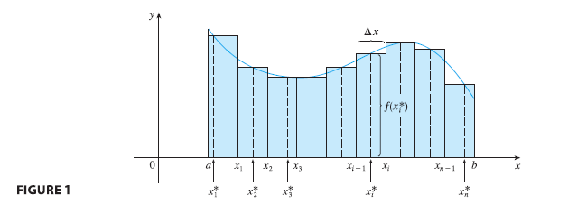
First let’s recall the basic facts concerning definite integrals of functions of a single variable. If \(f(x)\) is defined for \(a \le x \le b\), we start by dividing the interval \([a, b]\) into \(n\) subintervals \([x_{i-1}, x_i]\) of equal width \(\Delta x = (b - a)/n\) and we choose sample points \(x_i^*\) in these subintervals. Then we form the Riemann sum \[ \sum_{i=1}^{n} f(x_i^*) \Delta x \tag{1} \] and take the limit of such sums as \(n \to \infty\) to obtain the definite integral of \(f\) from \(a\) to \(b\):
\[ \int_a^b f(x) dx = \lim_{n \to \infty} \sum_{i=1}^{n} f(x_i^*) \Delta x \tag{2} \] In the special case where \(f(x) \ge 0\), the Riemann sum can be interpreted as the sum of the areas of the approximating rectangles in Figure 1, and \(\int_a^b f(x) dx\) represents the area under the curve \(y = f(x)\) from \(a\) to \(b\).
Volumes and Double Integrals
We consider a function \(f\) of two variables defined on a closed rectangle \[ R = [a, b] \times [c, d] = \{(x, y) \in \mathbb{R}^2 | a \le x \le b, c \le y \le d\} \] and we first suppose that \(f(x, y) \ge 0\). The graph of \(f\) is a surface with equation \(z = f(x, y)\).
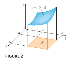
Let \(S\) be the solid that lies above \(R\) and under the graph of \(f\), that is, \[ S = \{(x, y, z) \in \mathbb{R}^3 | 0 \le z \le f(x, y), (x, y) \in R\} \] (See Figure 2.) Our goal is to find the volume of \(S\).
The first step is to divide the rectangle \(R\) into subrectangles. We accomplish this by dividing the interval \([a, b]\) into \(m\) subintervals \([x_{i-1}, x_i]\) of equal width \(\Delta x = (b - a)/m\) and dividing \([c, d]\) into \(n\) subintervals \([y_{j-1}, y_j]\) of equal width \(\Delta y = (d - c)/n\). By drawing lines parallel to the coordinate axes through the endpoints of these subintervals, as in Figure 3, we form the subrectangles

\[ R_{ij} = [x_{i-1}, x_i] \times [y_{j-1}, y_j] = \{(x, y) | x_{i-1} \le x \le x_i, y_{j-1} \le y \le y_j\} \] each with area \(\Delta A = \Delta x \Delta y\).
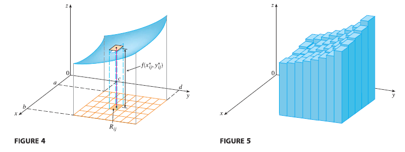
If we choose a sample point \((x_{ij}^*, y_{ij}^*)\) in each \(R_{ij}\), then we can approximate the part of \(S\) that lies above each \(R_{ij}\) by a thin rectangular box (or “column”) with base \(R_{ij}\) and height \(f(x_{ij}^*, y_{ij}^*)\) as shown in Figure 4. The volume of this box is the height of the box times the area of the base rectangle: \[ f(x_{ij}^*, y_{ij}^*) \Delta A \]
If we follow this procedure for all the rectangles and add the volumes of the corresponding boxes, we get an approximation to the total volume of \(S\):
\[ \tag{3} V \approx \sum_{i=1}^{m} \sum_{j=1}^{n} f(x_{ij}^*, y_{ij}^*) \Delta A \]
(See Figure 5.) This double sum means that for each subrectangle we evaluate \(f\) at the chosen point and multiply by the area of the subrectangle, and then we add the results.
Our intuition tells us that the approximation given in (Eq 3) becomes better as \(m\) and \(n\) become larger and so we would expect that
\[ \tag{4} V = \lim_{m, n \to \infty} \sum_{i=1}^{m} \sum_{j=1}^{n} f(x_{ij}^*, y_{ij}^*) \Delta A \]
We use the expression in Equation (4) to define the volume of the solid \(S\) that lies under the graph of \(f\) and above the rectangle \(R\).
This dicussion leads to the following definition.
Definition The double integral of \(f\) over the rectangle \(R\) is \[ \tag{5} \iint_R f(x, y) dA = \lim_{m, n \to \infty} \sum_{i=1}^{m} \sum_{j=1}^{n} f(x_{ij}^*, y_{ij}^*) \Delta A \] if this limit exists.
The precise meaning of the limit in Definition 5 is that for every number \(\varepsilon > 0\) there is an integer \(N\) such that \[ \left| \iint_R f(x, y) dA - \sum_{i=1}^{m} \sum_{j=1}^{n} f(x_{ij}^*, y_{ij}^*) \Delta A \right| < \varepsilon \] for all integers \(m\) and \(n\) greater than \(N\) and for any choice of sample points \((x_{ij}^*, y_{ij}^*)\) in \(R_{ij}\).
A function \(f\) is called integrable if the limit in Definition exists.
- It is shown in courses on advanced calculus that all continuous functions are integrable. In fact, the double integral of \(f\) exists provided that \(f\) is “not too discontinuous.” In particular, if \(f\) is bounded on \(R\), [that is, there is a constant \(M\) such that \(|f(x, y)| \le M\) for all \((x, y)\) in \(R\)], and \(f\) is continuous there, except on a finite number of smooth curves, then \(f\) is integrable over \(R\).
The sample point \((x_{ij}^*, y_{ij}^*)\) can be chosen to be any point in the subrectangle \(R_{ij}\), but if we choose it to be the upper right-hand corner of \(R_{ij}\) [namely \((x_i, y_j)\), see Figure 3], then the expression for the double integral looks simpler:
\[ \tag{6} \iint_R f(x, y) dA = \lim_{m, n \to \infty} \sum_{i=1}^{m} \sum_{j=1}^{n} f(x_i, y_j) \Delta A \]
We see that a volume can be written as a double integral:
If \(f(x, y) \ge 0\), then the volume \(V\) of the solid that lies above the rectangle \(R\) and below the surface \(z = f(x, y)\) is \[ V = \iint_R f(x, y) dA \]
The sum in Definition 5, \[ \sum_{i=1}^{m} \sum_{j=1}^{n} f(x_{ij}^*, y_{ij}^*) \Delta A \] is called a double Riemann sum and is used as an approximation to the value of the double integral. If \(f\) happens to be a positive function, then the double Riemann sum represents the sum of volumes of columns, as in Figure 5, and is an approximation to the volume under the graph of \(f\).
Example
EXAMPLE 2 If \(R = \{(x, y) | -1 \le x \le 1, -2 \le y \le 2\}\), evaluate the integral \(\iint_R \sqrt{1 - x^2} dA\).
The Midpoint Rule
The methods that we used for approximating single integrals (the Midpoint Rule, the Trapezoidal Rule, Simpson’s Rule) all have counterparts for double integrals. Here we consider only the Midpoint Rule for double integrals. This means that we use a double Riemann sum to approximate the double integral, where the sample point \((x_{ij}^*, y_{ij}^*)\) in \(R_{ij}\) is chosen to be the center \((\bar{x}_i, \bar{y}_j)\) of \(R_{ij}\). In other words, \(\bar{x}_i\) is the midpoint of \([x_{i-1}, x_i]\) and \(\bar{y}_j\) is the midpoint of \([y_{j-1}, y_j]\).
Midpoint Rule for Double Integrals \[ \iint_R f(x, y) dA \approx \sum_{i=1}^{m} \sum_{j=1}^{n} f(\bar{x}_i, \bar{y}_j) \Delta A \] where \(\bar{x}_i\) is the midpoint of \([x_{i-1}, x_i]\) and \(\bar{y}_j\) is the midpoint of \([y_{j-1}, y_j]\).
Example: midpoint rule
EXAMPLE 3 Use the Midpoint Rule with \(m = n = 2\) to estimate the value of the integral \(\iint_R (x - 3y^2) dA\), where \(R = \{(x, y) | 0 \le x \le 2, 1 \le y \le 2\}\).
Iterated Integrals
Recall that it is usually difficult to evaluate single integrals directly from the definition of an integral, but the Fundamental Theorem of Calculus provides a much easier method. The evaluation of double integrals from first principles is even more difficult, but here we see how to express a double integral as an iterated integral, which can then be evaluated by calculating two single integrals.
Suppose that \(f\) is a function of two variables that is integrable on the rectangle \(R = [a, b] \times [c, d]\). We use the notation \(\int_c^d f(x, y) dy\) to mean that \(x\) is held fixed and \(f(x, y)\) is integrated with respect to \(y\) from \(y = c\) to \(y = d\). This procedure is called partial integration with respect to y. Now \(\int_c^d f(x, y) dy\) is a number that depends on the value of \(x\), so it defines a function of \(x\): \[ A(x) = \int_c^d f(x, y) dy \] If we now integrate the function \(A\) with respect to \(x\) from \(x = a\) to \(x = b\), we get
\[ \tag{7} \int_a^b A(x) dx = \int_a^b \left[ \int_c^d f(x, y) dy \right] dx \]
The integral on the right side of Equation (7)) is called an iterated integral. Usually the brackets are omitted. Thus
\[ \tag{8} \int_a^b \int_c^d f(x, y) dy dx = \int_a^b \left[ \int_c^d f(x, y) dy \right] dx \] means that we first integrate with respect to \(y\) from \(c\) to \(d\) and then with respect to \(x\) from \(a\) to \(b\).
Similarly, the iterated integral \[ \tag{eq:9} \int_c^d \int_a^b f(x, y) dx dy = \int_c^d \left[ \int_a^b f(x, y) dx \right] dy \] means that we first integrate with respect to \(x\) (holding \(y\) fixed) from \(x = a\) to \(x = b\) and then we integrate the resulting function of \(y\) with respect to \(y\) from \(y = c\) to \(y = d\).
Notice that in both Equations (8) and (9) we work from the inside out.
Example - Iterated Integrals
EXAMPLE 4 Evaluate the iterated integrals. (a) \(\int_0^3 \int_1^2 x^2y dy dx\) (b) \(\int_1^2 \int_0^3 x^2y dx dy\)
Fubini's Theorem
The following theorem gives a practical method for evaluating a double integral by expressing it as an iterated integral (in either order).
10 Fubini’s Theorem If \(f\) is continuous on the rectangle \(R = \{(x, y) | a \le x \le b, c \le y \le d\}\), then \[ \iint_R f(x, y) dA = \int_a^b \int_c^d f(x, y) dy dx = \int_c^d \int_a^b f(x, y) dx dy \] More generally, this is true if we assume that \(f\) is bounded on \(R\), \(f\) is discontinuous only on a finite number of smooth curves, and the iterated integrals exist.
More Example
EXAMPLE 5 Evaluate the double integral \(\iint_R (x - 3y^2) dA\), where \(R = \{(x, y) | 0 \le x \le 2, 1 \le y \le 2\}\).
Example
EXAMPLE 6 Evaluate \(\iint_R y \sin(xy) dA\), where \(R = [1, 2] \times [0, \pi]\).
Example
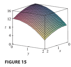
EXAMPLE 7 Find the volume of the solid \(S\) that is bounded by the elliptic paraboloid \(x^2 + 2y^2 + z = 16\), the planes \(x = 2\) and \(y = 2\), and the three coordinate planes.
Average Value
Recall from one variable calculs that the average value of a functio \(f\) of one variable defined on an interval \([a, b]\) is \[ f_{ave} = \frac{1}{b-a} \int_a^b f(x) dx \] In a similar fashion we define the average value of a function \(f\) of two variables defined on a rectangle \(R\) to be \[ f_{ave} = \frac{1}{A(R)} \iint_R f(x, y) dA \] where \(A(R)\) is the area of \(R\). If \(f(x, y) \ge 0\), the equation \[ A(R) \times f_{ave} = \iint_R f(x, y) dA \] says that the box with base \(R\) and height \(f_{ave}\) has the same volume as the solid that lies under the graph of \(f\).
Exercise 1
- Estimate the volume of the solid that lies below the surface \(z = xy\) and above the rectangle \(R = \{(x, y) | 0 \le x \le 6, 0 \le y \le 4\}\). Use a Riemann sum with \(m = 3\), \(n = 2\), and take the sample point to be the upper right corner of each square.
- Use the Midpoint Rule to estimate the volume of the solid in part (a).
Exercise 2
If \(R = [0, 4] \times [-1, 2]\), use a Riemann sum with \(m = 2\), \(n = 3\) to estimate the value of \(\iint_R (1 - xy^2) dA\). Take the sample points to be (a) the lower right corners and (b) the upper left corners of the rectangles.
Exercise 3
- Use a Riemann sum with \(m = n = 2\) to estimate the value of \(\iint_R xe^{-xy} dA\), where \(R = [0, 2] \times [0, 1]\). Take the sample points to be upper right corners.
- Use the Midpoint Rule to estimate the integral in part (a).
Exercise 4
- Estimate the volume of the solid that lies below the surface \(z = 1 + x^2 + 3y\) and above the rectangle \(R = [1, 2] \times [0, 3]\). Use a Riemann sum with \(m = n = 2\) and choose the sample points to be lower left corners.
- Use the Midpoint Rule to estimate the volume in part (a).
Exercise 5
Let V be the volume of the solid that lies under the graph of \(f(x, y) = \sqrt{52 - x^2 - y^2}\) and above the rectangle given by \(2 \le x \le 4\), \(2 \le y \le 6\). Use the lines \(x = 3\) and \(y = 4\) to divide R into subrectangles. Let L and U be the Riemann sums computed using lower left corners and upper right corners, respectively. Without calculating the numbers V, L, and U, arrange them in increasing order and explain your reasoning.
Exercise 6
A 20-ft-by-30-ft swimming pool is filled with water. The depth is
measured at 5-ft intervals, starting at one corner of the pool, and the
values are recorded in the table. Estimate the volume of water in the
pool. 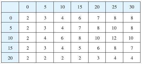
Exercise 7
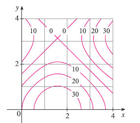
A contour map is shown for a function \(f\) on the square \(R = [0, 4] \times [0, 4]\). (a) Use the Midpoint Rule with \(m = n = 2\) to estimate the value of \(\iint_R f(x, y) dA\). (b) Estimate the average value of \(f\).
Exercise 8
The contour map shows the temperature, in degrees Fahrenheit, at 4:00 PM on February 26, 2007, in Colorado. (The state measures 388 mi west to east and 276 mi south to north.) Use the Midpoint Rule with \(m = n = 4\) to estimate the average temperature in Colorado at that time.
Exercise 9
Evaluate the double integral \(\iint_R \sqrt{2} dA\), where \(R = \{(x, y) | 2 \le x \le 6, -1 \le y \le 5\}\) by first identifying it as the volume of a solid.
Exercise 10
Evaluate the double integral \(\iint_R (2x + 1) dA\), where \(R = \{(x, y) | 0 \le x \le 2, 0 \le y \le 4\}\) by first identifying it as the volume of a solid.
Exercise 11
Evaluate the double integral \(\iint_R (4 - 2y) dA\), where \(R = [0, 1] \times [0, 1]\) by first identifying it as the volume of a solid.
Exercise 12
The integral \(\iint_R \sqrt{9 - y^2} dA\), where \(R = [0, 4] \times [0, 2]\), represents the volume of a solid. Sketch the solid.
Exercise 13
Find \(\int_0^5 f(x, y) dx\) and \(\int_0^1 f(x, y) dy\) for \(f(x, y) = x + 3x^2y^2\).
Exercise 14
Find \(\int_0^5 f(x, y) dx\) and \(\int_0^1 f(x, y) dy\) for \(f(x, y) = y\sqrt{x} + 2\).
Exercise 15
Calculate the iterated integral \(\int_1^4 \int_0^2 (6x^2y - 2x) dy dx\).
Exercise 16
Calculate the iterated integral \(\int_0^1 \int_1^2 (x + e^{-y})^2 dx dy\).
Exercise 17
Calculate the iterated integral \(\int_0^1 \int_0^1 (x + e^y) dx dy\).
Exercise 18
Calculate the iterated integral \(\int_0^{\pi/6} \int_0^{\pi/2} (\sin x + \sin y) dy dx\).
Exercise 19
Calculate the iterated integral \(\int_0^3 \int_{-2}^0 (y^2 + y^3 \cos x) dx dy\).
Exercise 20
Calculate the iterated integral \(\int_1^4 \int_1^2 (\frac{x}{y} + \frac{y}{x}) dy dx\).
Exercise 21
Calculate the iterated integral \(\int_1^2 \int_0^1 \frac{x}{y} dy dx\).
Exercise 22
Calculate the iterated integral \(\int_0^1 \int_0^1 ye^{xy} dx dy\).
Exercise 23
Calculate the iterated integral \(\int_0^{\pi/2} \int_0^{\pi/2} \sin \theta \cos \phi d\theta d\phi\).
Exercise 24
Calculate the iterated integral \(\int_0^1 \int_0^1 xy\sqrt{x^2 + y^2} dy dx\).
Exercise 25
Calculate the iterated integral \(\int_0^1 \int_0^1 \sqrt{u + v^2} du dv\).
Exercise 26
Calculate the iterated integral \(\int_0^1 \int_0^1 \frac{1}{\sqrt{s+t}} ds dt\).
Exercise 27
Calculate the double integral \(\iint_R x \sec^2 y dA\), where \(R = \{(x, y) | 0 \le x \le 2, 0 \le y \le \pi/4\}\).
Exercise 28
Calculate the double integral \(\iint_R (y + xy^{-2}) dA\), where \(R = \{(x, y) | 0 \le x \le 2, 1 \le y \le 2\}\).
Exercise 29
Calculate the double integral \(\iint_R \frac{xy^2}{x^2 + 1} dA\), where \(R = \{(x, y) | 0 \le x \le 1, -3 \le y \le 3\}\).
Exercise 30
Calculate the double integral \(\iint_R \frac{\tan \theta}{\sqrt{1 - t^2}} dA\), where \(R = \{(\theta, t) | 0 \le \theta \le \pi/3, 0 \le t \le 1/2\}\).
Exercise 31
Calculate the double integral \(\iint_R x \sin(x + y) dA\), where \(R = [0, \pi/6] \times [0, \pi/3]\).
Exercise 32
Calculate the double integral \(\iint_R \frac{x}{1 + xy} dA\), where \(R = [0, 1] \times [0, 1]\).
Exercise 33
Calculate the double integral \(\iint_R ye^{xy} dA\), where \(R = [0, 2] \times [0, 3]\).
Exercise 34
Calculate the double integral \(\iint_R \frac{1}{1 + x + y} dA\), where \(R = [1, 3] \times [1, 2]\).
Exercise 35
Sketch the solid whose volume is given by the iterated integral \(\int_0^1 \int_0^1 (4 - x - 2y) dx dy\).
Exercise 36
Sketch the solid whose volume is given by the iterated integral \(\int_0^1 \int_0^1 (2 - x^2 - y^2) dy dx\).
Exercise 37
Find the volume of the solid that lies under the plane \(4x + 6y - 2z + 15 = 0\) and above the rectangle \(R = \{(x, y) | -1 \le x \le 2, -1 \le y \le 1\}\).
Exercise 38
Find the volume of the solid that lies under the hyperbolic paraboloid \(z = 3y^2 - x^2 + 2\) and above the rectangle \(R = [-1, 1] \times [1, 2]\).
Exercise 39
Find the volume of the solid lying under the elliptic paraboloid \(x^2/4 + y^2/9 + z = 1\) and above the rectangle \(R = [-1, 1] \times [-2, 2]\).
Exercise 40
Find the volume of the solid enclosed by the surface \(z = x^2 + xy^2\) and the planes \(z = 0, x = 0, x = 5,\) and \(y = \pm 2\).
Exercise 41
Find the volume of the solid enclosed by the surface \(z = 1 + e^x \sin y\) and the planes \(z = 0, x = \pm 1, y = 0,\) and \(y = \pi\).
Exercise 42
Find the volume of the solid in the first octant bounded by the cylinder \(z = 16 - x^2\) and the plane \(y = 5\).
Exercise 43
Find the volume of the solid enclosed by the paraboloid \(z = 2 + x^2 + (y - 2)^2\) and the planes \(z = 1, x = 1, x = -1, y = 0,\) and \(y = 4\).
Exercise 44
Graph the solid that lies between the surface \(z = 2xy/(x^2 + 1)\) and the plane \(z = x + 2y\) and is bounded by the planes \(x = 0, x = 2, y = 0,\) and \(y = 4\). Then find its volume.
Exercise 45
Use a computer algebra system to find the exact value of the integral \(\iint_R x^5y^3e^{xy} dA\), where \(R = [0, 1] \times [0, 1]\). Then use the CAS to draw the solid whose volume is given by the integral.
Exercise 46
Graph the solid that lies between the surfaces \(z = e^{-x^2} \cos(x^2 + y^2)\) and \(z = 2 - x^2 - y^2\) for \(|x| \le 1, |y| \le 1\). Use a computer algebra system to approximate the volume of this solid correct to four decimal places.
Exercise 47
Find the average value of \(f(x, y) = x^2y\) over the rectangle R with vertices \((-1, 0), (-1, 5), (1, 5), (1, 0)\).
Exercise 48
Find the average value of \(f(x, y) = e^y\sqrt{x + e^y}\) over the rectangle \(R = [0, 4] \times [0, 1]\).
Exercise 49
Use symmetry to evaluate the double integral \(\iint_R \frac{xy}{1 + x^4} dA\), where \(R = \{(x, y) | -1 \le x \le 1, 0 \le y \le 1\}\).
Exercise 50
Use symmetry to evaluate the double integral \(\iint_R (1 + x^2 \sin y + y^2 \sin x) dA\), where \(R = [-\pi, \pi] \times [-\pi, \pi]\).
Exercise 51
Use a CAS to compute the iterated integrals \(\int_0^1 \int_0^1 \frac{x - y}{(x + y)^3} dy dx\) and \(\int_0^1 \int_0^1 \frac{x - y}{(x + y)^3} dx dy\). Do the answers contradict Fubini’s Theorem? Explain what is happening.
Exercise 52
- In what way are the theorems of Fubini and Clairaut similar?
- If \(f(x, y)\) is continuous on \([a, b] \times [c, d]\) and \(g(x, y) = \int_a^x \int_c^y f(s, t) dt ds\) for \(a < x < b, c < y < d\), show that \(g_{xy} = g_{yx} = f(x, y)\).