Section 13.1: Vector Functions and Space Curves
| Site: | Freebirds Moodle |
| Course: | Mathematical Methods I - SNIOE - Monsoon 2025 |
| Book: | Section 13.1: Vector Functions and Space Curves |
| Printed by: | Guest user |
| Date: | Monday, 9 February 2026, 8:11 AM |
Table of contents
- Vector Functions
- Limits and Continuity of vector function
- Space Curves
- Example problem
- Using Computers to Draw Space Curves
- Exercise 1
- Exercise 2
- Exercise 3
- Exercise 4
- Exercise 5
- Exercise 6
- Exercise 7
- Exercise 8
- Exercise 9
- Exercise 10
- Exercise 11
- Exercise 12
- Exercise 13
- Exercise 14
- Exercise 15
- Exercise 16
- Exercise 17
- Exercise 18
- Exercise 19
- Exercise 20
- Exercise 21
- Exercise 22
- Exercise 23
- Exercise 24
- Exercise 25
- Exercise 26
- Exercise 27
- Exercise 28
- Exercise 29
- Exercise 30
- Exercise 31
- Exercise 32
- Exercise 33
- Exercise 34
- Exercise 35
- Exercise 36
- Exercise 37
- Exercise 38
- Exercise 39
- Exercise 40
- Exercise 41
- Exercise 42
- Exercise 43
- Exercise 44
- Exercise 45
- Exercise 46
- Exercise 47
- Exercise 48
- Exercise 49
- Exercise 50
- Exercise 51
- Exercise 52
- Exercise 53
- Exercise 54
Vector Functions
In general, a function is a rule that assigns to each element in the domain an element in the range. A vector-valued function, or vector function, is simply a function whose domain is a set of real numbers and whose range is a set of vectors. We are most interested in vector functions r whose values are three-dimensional vectors. This means that for every number \(t\) in the domain of r there is a unique vector in \(V_3\) denoted by \(\mathbf{r}(t)\). If \(f(t)\), \(g(t)\), and \(h(t)\) are the components of the vector \(\mathbf{r}(t)\), then \(f\), \(g\), and \(h\) are real-valued functions called the component functions of r and we can write \[ \mathbf{r}(t) = \langle f(t), g(t), h(t) \rangle = f(t)\mathbf{i} + g(t)\mathbf{j} + h(t)\mathbf{k} \] We use the letter \(t\) to denote the independent variable because it represents time in most applications of vector functions.
EXAMPLE 1 If \[ \mathbf{r}(t) = \langle t^3, \ln(3-t), \sqrt{t} \rangle \] then the component functions are \[ f(t) = t^3 \qquad g(t) = \ln(3-t) \qquad h(t) = \sqrt{t} \] By our usual convention, the domain of r consists of all values of \(t\) for which the expression for \(\mathbf{r}(t)\) is defined. The expressions \(t^3\), \(\ln(3-t)\), and \(\sqrt{t}\) are all defined when \(3-t > 0\) and \(t \ge 0\). Therefore the domain of r is the interval \([0, 3)\).
Limits and Continuity of vector function
The limit of a vector function r is defined by taking the limits of its component functions as follows.
- If \(\mathbf{r}(t) = \langle f(t), g(t), h(t) \rangle\), then \[ \lim_{t \to a} \mathbf{r}(t) = \left\langle \lim_{t \to a} f(t), \lim_{t \to a} g(t), \lim_{t \to a} h(t) \right\rangle \] provided the limits of the component functions exist.
If \(\lim_{t \to a} \mathbf{r}(t) = \mathbf{L}\), this definition is equivalent to saying that the length and direction of the vector \(\mathbf{r}(t)\) approach the length and direction of the vector L.
Equivalently, we could have used an \(\epsilon-\delta\) definition (see Exercise 54). Limits of vector functions obey the same rules as limits of real-valued functions (see Exercise 53).
EXAMPLE 2 Find \(\lim_{t \to 0} \mathbf{r}(t)\), where \(\mathbf{r}(t) = (1+t^3)\mathbf{i} + te^{-t}\mathbf{j} + \frac{\sin t}{t}\mathbf{k}\).
A vector function r is continuous at a if \[ \lim_{t \to a} \mathbf{r}(t) = \mathbf{r}(a) \] In view of Definition 1, we see that r is continuous at \(a\) if and only if its component functions \(f\), \(g\), and \(h\) are continuous at \(a\).
Space Curves
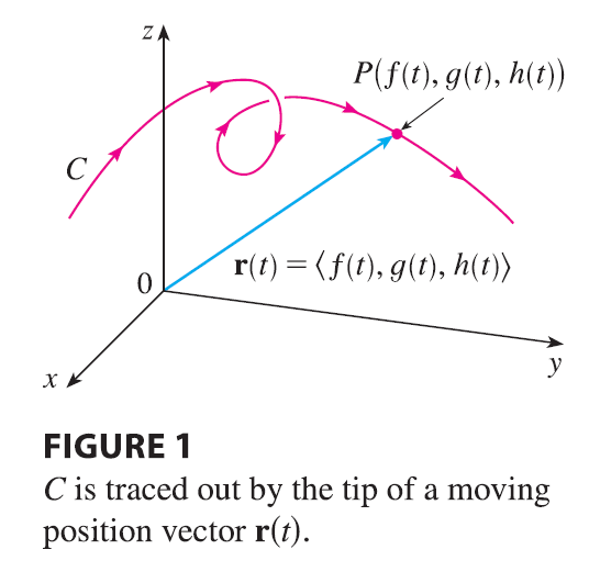
There is a close connection between continuous vector functions and space curves. Suppose that \(f\), \(g\), and \(h\) are continuous real-valued functions on an interval \(I\). Then the set \(C\) of all points \((x, y, z)\) in space, where \[ x = f(t) \quad y = g(t) \quad z = h(t) \tag{2} \] and \(t\) varies throughout the interval \(I\), is called a space curve. The equations in (2) are called parametric equations of \(C\) and \(t\) is called a parameter. We can think of \(C\) as being traced out by a moving particle whose position at time \(t\) is \((f(t), g(t), h(t))\). If we now consider the vector function \(\mathbf{r}(t) = \langle f(t), g(t), h(t) \rangle\), then \(\mathbf{r}(t)\) is the position vector of the point \(P(f(t), g(t), h(t))\) on \(C\). Thus any continuous vector function r defines a space curve \(C\) that is traced out by the tip of the moving vector \(\mathbf{r}(t)\), as shown in Figure 1.
EXAMPLE 3 Describe the curve defined by the vector function \[ \mathbf{r}(t) = \langle 1+t, 2+5t, -1+6t \rangle \]
Plane curves can also be represented in vector notation. For instance, the curve given by the parametric equations \(x = t^2 - 2t\) and \(y = t+1\) could also be described by the vector equation \[ \mathbf{r}(t) = \langle t^2 - 2t, t+1 \rangle = (t^2 - 2t)\mathbf{i} + (t+1)\mathbf{j} \] where \(\mathbf{i} = \langle 1, 0 \rangle\) and \(\mathbf{j} = \langle 0, 1 \rangle\).
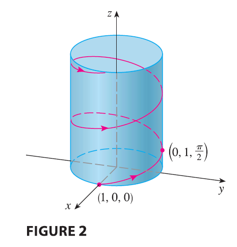
EXAMPLE 4 Sketch the curve whose vector equation is \[ \mathbf{r}(t) = \cos t \mathbf{i} + \sin t \mathbf{j} + t \mathbf{k} \]
The corkscrew shape of the helix in Example 4 is familiar from its occurrence in coiled springs. It also occurs in the model of DNA (deoxyribonucleic acid, the genetic material of living cells). In 1953 James Watson and Francis Crick showed that the structure of the DNA molecule is that of two linked, parallel helixes that are intertwined as in Figure 3.

Example problem
In Examples 3 and 4 we were given vector equations of curves and asked for a geometric description or sketch. In the next two examples we are given a geometric description of a curve and are asked to find parametric equations for the curve.
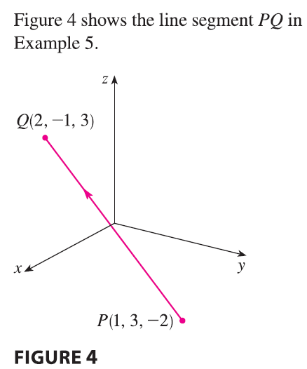
EXAMPLE 5 Find a vector equation and parametric equations for the line segment that joins the point \(P(1, 3, -2)\) to the point \(Q(2, -1, 3)\).
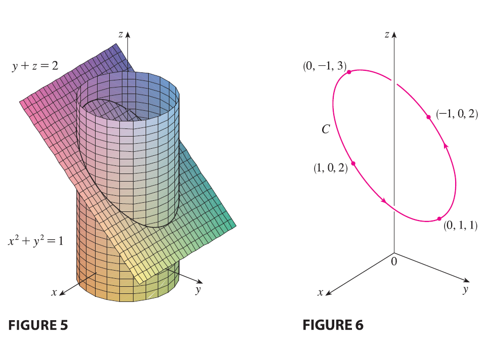
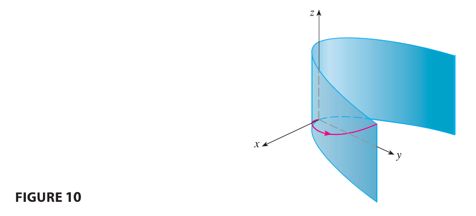
EXAMPLE 6 Find a vector function that represents the curve of intersection of the cylinder \(x^2 + y^2 = 1\) and the plane \(y+z=2\).
Using Computers to Draw Space Curves
Space curves are inherently more difficult to draw by hand than plane curves; for an accurate representation we need to use technology. For instance, Figure 7 shows a computer-generated graph of the curve with parametric equations \[ x = (4 + \sin 20t)\cos t \qquad y = (4 + \sin 20t)\sin t \qquad z = \cos 20t \]
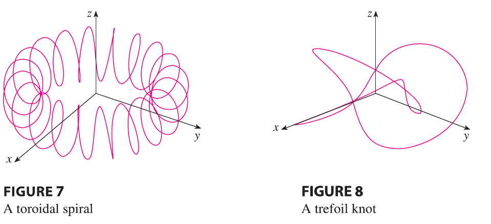
It’s called a toroidal spiral because it lies on a torus. Another interesting curve, the trefoil knot, with equations \[ x = (2 + \cos 1.5t)\cos t \qquad y = (2 + \cos 1.5t)\sin t \qquad z = \sin 1.5t \] is graphed in Figure 8. It wouldn’t be easy to plot either of these curves by hand.
Even when a computer is used to draw a space curve, optical illusions make it difficult to get a good impression of what the curve really looks like. (This is especially true in Figure 8. See Exercise 52.) The next example shows how to cope with this problem.
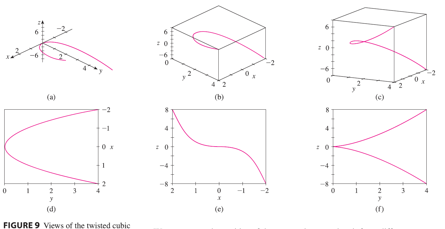
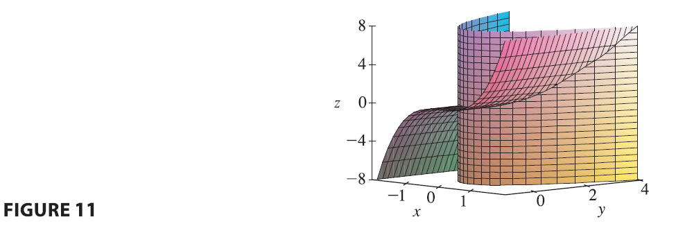
EXAMPLE 7 Use a computer to draw the curve with vector equation \(\mathbf{r}(t) = \langle t, t^2, t^3 \rangle\). This curve is called a twisted cubic.
Exercise 1
Find the domain of the vector function. \(\mathbf{r}(t) = \left\langle \ln(t+1), \frac{t}{\sqrt{9-t^2}}, 2^t \right\rangle\)
Exercise 2
Find the domain of the vector function. \(\mathbf{r}(t) = \cos t \mathbf{i} + \ln t \mathbf{j} + \frac{1}{t-2}\mathbf{k}\)
Exercise 3
Find the limit. \(\lim_{t \to 0} \left( e^{-3t}\mathbf{i} + \frac{t^2}{\sin^2 t}\mathbf{j} + \cos 2t \mathbf{k} \right)\)
Exercise 4
Find the limit. \(\lim_{t \to 1} \left( \frac{t^2-t}{t-1}\mathbf{i} + \sqrt{t+8}\mathbf{j} + \frac{\sin \pi t}{\ln t}\mathbf{k} \right)\)
Exercise 5
Find the limit. \(\lim_{t \to \infty} \left\langle \frac{1+t^2}{1-t^2}, \tan^{-1} t, \frac{1-e^{-2t}}{t} \right\rangle\)
Exercise 6
Find the limit. \(\lim_{t \to \infty} \left\langle te^{-t}, \frac{t^3+t}{2t^3-1}, t\sin\frac{1}{t} \right\rangle\)
Exercise 7
Sketch the curve with the given vector equation. Indicate with an arrow the direction in which t increases. \(\mathbf{r}(t) = \langle \sin \pi t, t \rangle\)
Exercise 8
Sketch the curve with the given vector equation. Indicate with an arrow the direction in which t increases. \(\mathbf{r}(t) = \langle t^2-1, t \rangle\)
Exercise 9
Sketch the curve with the given vector equation. Indicate with an arrow the direction in which t increases. \(\mathbf{r}(t) = \langle t, 2-t, 2t \rangle\)
Exercise 10
Sketch the curve with the given vector equation. Indicate with an arrow the direction in which t increases. \(\mathbf{r}(t) = \langle \sin \pi t, t, \cos \pi t \rangle\)
Exercise 11
Sketch the curve with the given vector equation. Indicate with an arrow the direction in which t increases. \(\mathbf{r}(t) = \langle 3, t, 2-t^2 \rangle\)
Exercise 12
Sketch the curve with the given vector equation. Indicate with an arrow the direction in which t increases. \(\mathbf{r}(t) = 2\cos t \mathbf{i} + 2\sin t \mathbf{j} + \mathbf{k}\)
Exercise 13
Sketch the curve with the given vector equation. Indicate with an arrow the direction in which t increases. \(\mathbf{r}(t) = t^2\mathbf{i} + t^4\mathbf{j} + t^6\mathbf{k}\)
Exercise 14
Sketch the curve with the given vector equation. Indicate with an arrow the direction in which t increases. \(\mathbf{r}(t) = \cos t \mathbf{i} - \cos t \mathbf{j} + \sin t \mathbf{k}\)
Exercise 15
Draw the projections of the curve on the three coordinate planes. Use these projections to help sketch the curve. \(\mathbf{r}(t) = \langle t, \sin t, 2\cos t \rangle\)
Exercise 16
Draw the projections of the curve on the three coordinate planes. Use these projections to help sketch the curve. \(\mathbf{r}(t) = \langle t, t, t^2 \rangle\)
Exercise 17
Find a vector equation and parametric equations for the line segment that joins P to Q. \(P(2, 0, 0), Q(6, 2, -2)\)
Exercise 18
Find a vector equation and parametric equations for the line segment that joins P to Q. \(P(-1, 2, -2), Q(-3, 5, 1)\)
Exercise 19
Find a vector equation and parametric equations for the line segment that joins P to Q. \(P(0, -1, 1), Q(\frac{1}{2}, \frac{1}{3}, \frac{1}{4})\)
Exercise 20
Find a vector equation and parametric equations for the line segment that joins P to Q. \(P(a, b, c), Q(u, v, w)\)
Exercise 21
Match the parametric equations with the graphs (labeled I-VI). Give reasons for your choices. \(x = t\cos t, y=t, z=t\sin t, t \ge 0\)

Exercise 22
Match the parametric equations with the graphs (labeled I-VI). Give reasons for your choices. \(x = \cos t, y=\sin t, z=1/(1+t^2)\)

Exercise 23
Match the parametric equations with the graphs (labeled I-VI). Give reasons for your choices. \(x=t, y=1/(1+t^2), z=t^2\)

Exercise 24
Match the parametric equations with the graphs (labeled I-VI). Give reasons for your choices. \(x=\cos t, y=\sin t, z=\cos 2t\)

Exercise 25
Match the parametric equations with the graphs (labeled I-VI). Give reasons for your choices. \(x=\cos 8t, y=\sin 8t, z=e^{0.8t}, t \ge 0\)
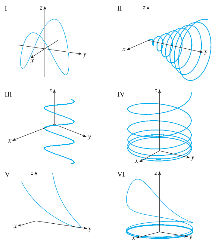
Exercise 26
Match the parametric equations with the graphs (labeled I-VI). Give reasons for your choices. \(x=\cos^2 t, y=\sin^2 t, z=t\)

Exercise 27
Show that the curve with parametric equations \(x = t \cos t, y = t \sin t, z = t\) lies on the cone \(z^2 = x^2 + y^2\), and use this fact to help sketch the curve.
Exercise 28
Show that the curve with parametric equations \(x = \sin t, y = \cos t, z = \sin^2 t\) is the curve of intersection of the surfaces \(z=x^2\) and \(x^2+y^2=1\). Use this fact to help sketch the curve.
Exercise 29
Find three different surfaces that contain the curve \(\mathbf{r}(t) = 2t\mathbf{i} + e^t\mathbf{j} + e^{2t}\mathbf{k}\).
Exercise 30
Find three different surfaces that contain the curve \(\mathbf{r}(t) = t^2\mathbf{i} + \ln t \mathbf{j} + (1/t)\mathbf{k}\).
Exercise 31
At what points does the curve \(\mathbf{r}(t) = t\mathbf{i} + (2t-t^2)\mathbf{k}\) intersect the paraboloid \(z=x^2+y^2\)?
Exercise 32
At what points does the helix \(\mathbf{r}(t) = \langle \sin t, \cos t, t \rangle\) intersect the sphere \(x^2+y^2+z^2=5\)?
Exercise 33
Use a computer to graph the curve with the given vector equation. Make sure you choose a parameter domain and viewpoints that reveal the true nature of the curve. \(\mathbf{r}(t) = \langle \cos t \sin 2t, \sin t \sin 2t, \cos 2t \rangle\)
Exercise 34
Use a computer to graph the curve with the given vector equation. Make sure you choose a parameter domain and viewpoints that reveal the true nature of the curve. \(\mathbf{r}(t) = \langle te^t, e^{-t}, t \rangle\)
Exercise 35
Use a computer to graph the curve with the given vector equation. Make sure you choose a parameter domain and viewpoints that reveal the true nature of the curve. \(\mathbf{r}(t) = \langle \sin 3t \cos t, \frac{1}{4}t, \sin 3t \sin t \rangle\)
Exercise 36
Use a computer to graph the curve with the given vector equation. Make sure you choose a parameter domain and viewpoints that reveal the true nature of the curve. \(\mathbf{r}(t) = \langle \cos(8\cos t)\sin t, \sin(8\cos t)\sin t, \cos t \rangle\)
Exercise 37
Use a computer to graph the curve with the given vector equation. Make sure you choose a parameter domain and viewpoints that reveal the true nature of the curve. \(\mathbf{r}(t) = \langle \cos 2t, \cos 3t, \cos 4t \rangle\)
Exercise 38
Graph the curve with parametric equations \(x = \sin t, y = \sin 2t, z = \cos 4t\). Explain its shape by graphing its projections onto the three coordinate planes.
Exercise 39
Graph the curve with parametric equations \(x = (1+\cos 16t)\cos t\) \(y = (1+\cos 16t)\sin t\) \(z = 1+\cos 16t\) Explain the appearance of the graph by showing that it lies on a cone.
Exercise 40
Graph the curve with parametric equations \(x = \sqrt{1-0.25\cos^2 10t}\cos t\) \(y = \sqrt{1-0.25\cos^2 10t}\sin t\) \(z = 0.5\cos 10t\) Explain the appearance of the graph by showing that it lies on a sphere.
Exercise 41
Show that the curve with parametric equations \(x=t^2, y=1-3t, z=1+t^3\) passes through the points \((1, -2, 2)\) and \((9, -8, 28)\) but not through the point \((4, 7, -6)\).
Exercise 42
Find a vector function that represents the curve of intersection of the two surfaces. The cylinder \(x^2+y^2=4\) and the surface \(z=xy\).
Exercise 43
Find a vector function that represents the curve of intersection of the two surfaces. The cone \(z=\sqrt{x^2+y^2}\) and the plane \(z=1+y\).
Exercise 44
Find a vector function that represents the curve of intersection of the two surfaces. The paraboloid \(z=4x^2+y^2\) and the parabolic cylinder \(y=x^2\).
Exercise 45
Find a vector function that represents the curve of intersection of the two surfaces. The hyperboloid \(z=x^2-y^2\) and the cylinder \(x^2+y^2=1\).
Exercise 46
Find a vector function that represents the curve of intersection of the two surfaces. The semiellipsoid \(x^2+y^2+4z^2=4, y \ge 0\), and the cylinder \(x^2+z^2=1\).
Exercise 47
Try to sketch by hand the curve of intersection of the circular cylinder \(x^2+y^2=4\) and the parabolic cylinder \(z=x^2\). Then find parametric equations for this curve and use these equations and a computer to graph the curve.
Exercise 48
Try to sketch by hand the curve of intersection of the parabolic cylinder \(y=x^2\) and the top half of the ellipsoid \(x^2+4y^2+4z^2=16\). Then find parametric equations for this curve and use these equations and a computer to graph the curve.
Exercise 49
If two objects travel through space along two different curves, it’s often important to know whether they will collide. (Will a missile hit its moving target? Will two aircraft collide?) The curves might intersect, but we need to know whether the objects are in the same position at the same time. Suppose the trajectories of two particles are given by the vector functions \(\mathbf{r}_1(t) = \langle t^2, 7t-12, t^2 \rangle\) \(\mathbf{r}_2(t) = \langle 4t-3, t^2, 5t-6 \rangle\) for \(t \ge 0\). Do the particles collide?
Exercise 50
Two particles travel along the space curves \(\mathbf{r}_1(t) = \langle t, t^2, t^3 \rangle\) \(\mathbf{r}_2(t) = \langle 1+2t, 1+6t, 1+14t \rangle\) Do the particles collide? Do their paths intersect?
Exercise 51
- Graph the curve with parametric equations \(x = \frac{27}{26}\sin 8t - \frac{8}{39}\sin 18t\) \(y = -\frac{27}{26}\cos 8t + \frac{8}{39}\cos 18t\) \(z = \frac{144}{65}\sin 5t\)
- Show that the curve lies on the hyperboloid of one sheet \(144x^2+144y^2-25z^2=100\).
Exercise 52
The view of the trefoil knot shown in Figure 8 is accurate, but it doesn’t reveal the whole story. Use the parametric equations \(x = (2+\cos 1.5t)\cos t\) \(y = (2+\cos 1.5t)\sin t\) \(z = \sin 1.5t\) to sketch the curve by hand as viewed from above, with gaps indicating where the curve passes over itself. Start by showing that the projection of the curve onto the xy-plane has polar coordinates \(r=2+\cos 1.5t\) and \(\theta=t\), so \(r\) varies between 1 and 3. Then show that \(z\) has maximum and minimum values when the projection is halfway between \(r=1\) and \(r=3\). When you have finished your sketch, use a computer to draw the curve with viewpoint directly above and compare with your sketch. Then use the computer to draw the curve from several other viewpoints. You can get a better impression of the curve if you plot a tube with radius 0.2 around the curve.
Exercise 53
Suppose u and v are vector functions that possess limits as \(t \to a\) and let c be a constant. Prove the following properties of limits. (a) \(\lim_{t \to a} [\mathbf{u}(t) + \mathbf{v}(t)] = \lim_{t \to a} \mathbf{u}(t) + \lim_{t \to a} \mathbf{v}(t)\) (b) \(\lim_{t \to a} c\mathbf{u}(t) = c \lim_{t \to a} \mathbf{u}(t)\) (c) \(\lim_{t \to a} [\mathbf{u}(t) \cdot \mathbf{v}(t)] = \lim_{t \to a} \mathbf{u}(t) \cdot \lim_{t \to a} \mathbf{v}(t)\) (d) \(\lim_{t \to a} [\mathbf{u}(t) \times \mathbf{v}(t)] = \lim_{t \to a} \mathbf{u}(t) \times \lim_{t \to a} \mathbf{v}(t)\)
Exercise 54
Show that \(\lim_{t \to a} \mathbf{r}(t) = \mathbf{b}\) if and only if for every \(\epsilon > 0\) there is a number \(\delta > 0\) such that if \(0 < |t-a| < \delta\) then \(|\mathbf{r}(t) - \mathbf{b}| < \epsilon\)