Section 13.3: Arc Length & Curvature
| Site: | Freebirds Moodle |
| Course: | Mathematical Methods I - SNIOE - Monsoon 2025 |
| Book: | Section 13.3: Arc Length & Curvature |
| Printed by: | Guest user |
| Date: | Monday, 9 February 2026, 8:11 AM |
Table of contents
- Length of a Curve
- Arc Length Function
- Curvature
- The Normal and Binormal Vectors
- Section Summary
- Exercise 1
- Exercise 2
- Exercise 3
- Exercise 4
- Exercise 5
- Exercise 6
- Exercise 7
- Exercise 8
- Exercise 9
- Exercise 10
- Exercise 11
- Exercise 12
- Exercise 13
- Exercise 14
- Exercise 15
- Exercise 16
- Exercise 17
- Exercise 18
- Exercise 19
- Exercise 20
- Exercise 21
- Exercise 22
- Exercise 23
- Exercise 24
- Exercise 25
- Exercise 26
- Exercise 27
- Exercise 28
- Exercise 29
- Exercise 30
- Exercise 31
- Exercise 32
- Exercise 33
- Exercise 34
- Exercise 35
- Exercise 36
- Exercise 37
- Exercise 38
- Exercise 39
- Exercise 40
- Exercise 41
- Exercise 42
- Exercise 43
- Exercise 44
- Exercise 45
- Exercise 46
- Exercise 47
- Exercise 48
- Exercise 49
- Exercise 50
- Exercise 51
- Exercise 52
- Exercise 53
- Exercise 54
- Exercise 55
- Exercise 56
- Exercise 57
- Exercise 58
- Exercise 59
- Exercise 60
Length of a Curve
In Section 10.2 we defined the length of a plane curve with parametric equations \(x = f(t)\), \(y = g(t)\), \(a \le t \le b\), as the limit of lengths of inscribed polygons and, for the case where \(f'\) and \(g'\) are continuous, we arrived at the formula
\[ L = \int_a^b \sqrt{[f'(t)]^2 + [g'(t)]^2} dt = \int_a^b \sqrt{\left(\frac{dx}{dt}\right)^2 + \left(\frac{dy}{dt}\right)^2} dt \tag{1} \]
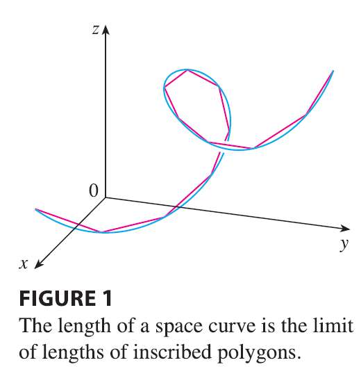
The length of a space curve is defined in exactly the same way (see Figure 1). Suppose that the curve has the vector equation \(\mathbf{r}(t) = \langle f(t), g(t), h(t) \rangle\), \(a \le t \le b\), or, equivalently, the parametric equations \(x = f(t)\), \(y = g(t)\), \(z = h(t)\), where \(f'\), \(g'\), and \(h'\) are continuous. If the curve is traversed exactly once as \(t\) increases from \(a\) to \(b\), then it can be shown that its length is
\[ L = \int_a^b \sqrt{[f'(t)]^2 + [g'(t)]^2 + [h'(t)]^2} dt \tag{2} \]
\[ = \int_a^b \sqrt{\left(\frac{dx}{dt}\right)^2 + \left(\frac{dy}{dt}\right)^2 + \left(\frac{dz}{dt}\right)^2} dt \]
Notice that both of the arc length formulas (1) and (2) can be put into the more compact form
\[ L = \int_a^b |\mathbf{r}'(t)| dt \tag{3} \]
because, for plane curves \(\mathbf{r}(t) = f(t)\mathbf{i} + g(t)\mathbf{j}\), \[ |\mathbf{r}'(t)| = |f'(t)\mathbf{i} + g'(t)\mathbf{j}| = \sqrt{[f'(t)]^2 + [g'(t)]^2} \] and for space curves \(\mathbf{r}(t) = f(t)\mathbf{i} + g(t)\mathbf{j} + h(t)\mathbf{k}\), \[ |\mathbf{r}'(t)| = |f'(t)\mathbf{i} + g'(t)\mathbf{j} + h'(t)\mathbf{k}| = \sqrt{[f'(t)]^2 + [g'(t)]^2 + [h'(t)]^2} \]
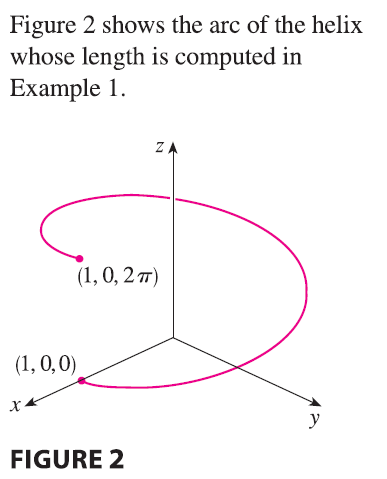
EXAMPLE 1 Find the length of the arc of the circular helix with vector equation \(\mathbf{r}(t) = \cos t \mathbf{i} + \sin t \mathbf{j} + t \mathbf{k}\) from the point \((1, 0, 0)\) to the point \((1, 0, 2\pi)\).
Arc Length Function
A single curve C can be represented by more than one vector function. For instance, the twisted cubic \[ \mathbf{r}_1(t) = \langle t, t^2, t^3 \rangle \qquad 1 \le t \le 2 \tag{4} \] could also be represented by the function \[ \mathbf{r}_2(u) = \langle e^u, e^{2u}, e^{3u} \rangle \qquad 0 \le u \le \ln 2 \tag{5} \] where the connection between the parameters \(t\) and \(u\) is given by \(t=e^u\). We say that Equations 4 and 5 are parametrizations of the curve C. If we were to use Equation 3 to compute the length of C using Equations 4 and 5, we would get the same answer. In general, it can be shown that when Equation 3 is used to compute arc length, the answer is independent of the parametrization that is used.
The Arc Length Function
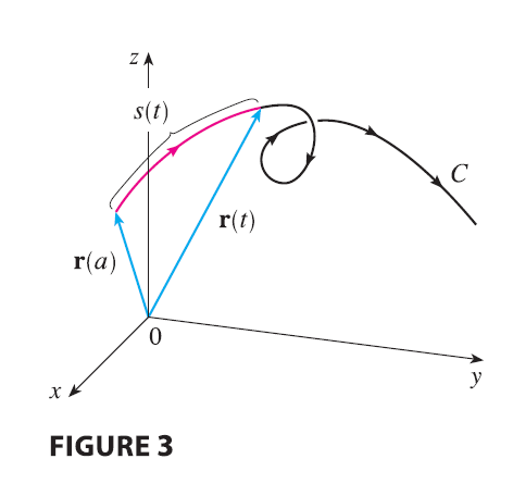
Now we suppose that C is a curve given by a vector function \[ \mathbf{r}(t) = f(t)\mathbf{i} + g(t)\mathbf{j} + h(t)\mathbf{k} \qquad a \le t \le b \] where \(\mathbf{r}'\) is continuous and C is traversed exactly once as \(t\) increases from \(a\) to \(b\). We define its arc length function s by
\[ s(t) = \int_a^t |\mathbf{r}'(u)| du = \int_a^t \sqrt{\left(\frac{dx}{du}\right)^2 + \left(\frac{dy}{du}\right)^2 + \left(\frac{dz}{du}\right)^2} du \tag{6} \]
Thus \(s(t)\) is the length of the part of C between \(\mathbf{r}(a)\) and \(\mathbf{r}(t)\). (See Figure 3.) If we differentiate both sides of Equation 6 using Part 1 of the Fundamental Theorem of Calculus, we obtain
\[ \frac{ds}{dt} = |\mathbf{r}'(t)| \tag{7} \]
It is often useful to parametrize a curve with respect to arc length because arc length arises naturally from the shape of the curve and does not depend on a particular coordinate system. If a curve \(\mathbf{r}(t)\) is already given in terms of a parameter \(t\) and \(s(t)\) is the arc length function given by Equation 6, then we may be able to solve for \(t\) as a function of \(s\): \(t = t(s)\). Then the curve can be reparametrized in terms of \(s\) by substituting for \(t\): \(\mathbf{r} = \mathbf{r}(t(s))\). Thus, if \(s=3\) for instance, \(\mathbf{r}(t(3))\) is the position vector of the point 3 units of length along the curve from its starting point.
EXAMPLE 2 Reparametrize the helix \(\mathbf{r}(t) = \cos t \mathbf{i} + \sin t \mathbf{j} + t \mathbf{k}\) with respect to arc length measured from \((1, 0, 0)\) in the direction of increasing \(t\).
Curvature
A parametrization \(\mathbf{r}(t)\) is called smooth on an interval I if \(\mathbf{r}'\) is continuous and \(\mathbf{r}'(t) \neq \mathbf{0}\) on I. A curve is called smooth if it has a smooth parametrization. A smooth curve has no sharp corners or cusps; when the tangent vector turns, it does so continuously.
If C is a smooth curve defined by the vector function \(\mathbf{r}\), recall that the unit tangent vector \(\mathbf{T}(t)\) is given by \[ \mathbf{T}(t) = \frac{\mathbf{r}'(t)}{|\mathbf{r}'(t)|} \]
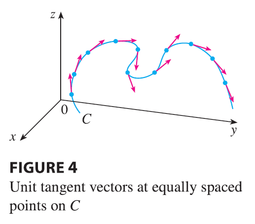
and indicates the direction of the curve. From Figure 4 you can see that \(\mathbf{T}(t)\) changes direction very slowly when C is fairly straight, but it changes direction more quickly when C bends or twists more sharply.
The curvature of C at a given point is a measure of how quickly the curve changes direction at that point. Specifically, we define it to be the magnitude of the rate of change of the unit tangent vector with respect to arc length. (We use arc length so that the curvature will be independent of the parametrization.) Because the unit tangent vector has constant length, only changes in direction contribute to the rate of change of \(\mathbf{T}\).
Definition 8 The curvature of a curve is \[ \kappa = \left| \frac{d\mathbf{T}}{ds} \right| \] where T is the unit tangent vector.
The curvature is easier to compute if it is expressed in terms of the parameter \(t\) instead of \(s\), so we use the Chain Rule (Theorem 13.2.3, Formula 6) to write \[ \frac{d\mathbf{T}}{dt} = \frac{d\mathbf{T}}{ds} \frac{ds}{dt} \quad \text{and} \quad \kappa = \left| \frac{d\mathbf{T}}{ds} \right| = \left| \frac{d\mathbf{T}/dt}{ds/dt} \right| \] But \(ds/dt = |\mathbf{r}'(t)|\) from Equation 7, so
\[ \kappa(t) = \frac{|\mathbf{T}'(t)|}{|\mathbf{r}'(t)|} \tag{9} \]
EXAMPLE 3 Show that the curvature of a circle of radius \(a\) is \(1/a\).
The result of Example 3 shows that small circles have large curvature and large circles have small curvature, in accordance with our intuition. We can see directly from the definition of curvature that the curvature of a straight line is always 0 because the tangent vector is constant.
Although Formula 9 can be used in all cases to compute the curvature, the formula given by the following theorem is often more convenient to apply.
Theorem 10 The curvature of the curve given by the vector function \(\mathbf{r}\) is \[ \kappa(t) = \frac{|\mathbf{r}'(t) \times \mathbf{r}''(t)|}{|\mathbf{r}'(t)|^3} \]
PROOF Since \(\mathbf{T} = \mathbf{r}'/|\mathbf{r}'|\) and \(|\mathbf{r}'| = ds/dt\), we have \[ \mathbf{r}' = |\mathbf{r}'|\mathbf{T} = \frac{ds}{dt}\mathbf{T} \] so the Product Rule (Theorem 13.2.3, Formula 3) gives \[ \mathbf{r}'' = \frac{d^2s}{dt^2}\mathbf{T} + \frac{ds}{dt}\mathbf{T}' \] Using the fact that \(\mathbf{T} \times \mathbf{T} = \mathbf{0}\), we have \[ \mathbf{r}' \times \mathbf{r}'' = \left(\frac{ds}{dt}\right)^2(\mathbf{T} \times \mathbf{T}') \] Now \(|\mathbf{T}(t)| = 1\) for all \(t\), so \(\mathbf{T}\) and \(\mathbf{T}'\) are orthogonal by Example 13.2.4. Therefore, by Theorem 12.4.9, \[ |\mathbf{r}' \times \mathbf{r}''| = \left(\frac{ds}{dt}\right)^2 |\mathbf{T} \times \mathbf{T}'| = \left(\frac{ds}{dt}\right)^2 |\mathbf{T}||\mathbf{T}'| = \left(\frac{ds}{dt}\right)^2 |\mathbf{T}'| \] Thus \[ |\mathbf{T}'| = \frac{|\mathbf{r}' \times \mathbf{r}''|}{(ds/dt)^2} = \frac{|\mathbf{r}' \times \mathbf{r}''|}{|\mathbf{r}'|^2} \] and \[ \kappa = \frac{|\mathbf{T}'|}{|\mathbf{r}'|} = \frac{|\mathbf{r}' \times \mathbf{r}''|}{|\mathbf{r}'|^3} \]
EXAMPLE 4 Find the curvature of the twisted cubic \(\mathbf{r}(t) = \langle t, t^2, t^3 \rangle\) at a general point and at \((0, 0, 0)\).
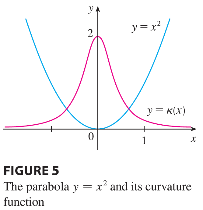
Curvature of graphs
For the special case of a plane curve with equation \(y=f(x)\), we choose \(x\) as the parameter and write \(\mathbf{r}(x) = x\mathbf{i} + f(x)\mathbf{j}\). Then \(\mathbf{r}'(x) = \mathbf{i} + f'(x)\mathbf{j}\) and \(\mathbf{r}''(x) = f''(x)\mathbf{j}\). Since \(\mathbf{i} \times \mathbf{j} = \mathbf{k}\) and \(\mathbf{j} \times \mathbf{j} = \mathbf{0}\), it follows that \(\mathbf{r}'(x) \times \mathbf{r}''(x) = f''(x)\mathbf{k}\). We also have \(|\mathbf{r}'(x)| = \sqrt{1+[f'(x)]^2}\) and so, by Theorem 10,
\[ \kappa(x) = \frac{|f''(x)|}{[1+(f'(x))^2]^{3/2}} \tag{11} \]
EXAMPLE 5 Find the curvature of the parabola \(y=x^2\) at the points \((0, 0)\), \((1, 1)\), and \((2, 4)\).
The Normal and Binormal Vectors
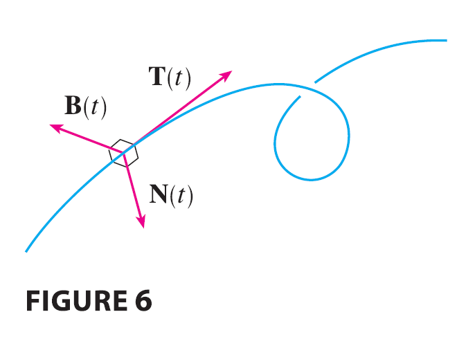
At a given point on a smooth space curve \(\mathbf{r}(t)\), there are many vectors that are orthogonal to the unit tangent vector \(\mathbf{T}(t)\). We single out one by observing that, because \(|\mathbf{T}(t)|=1\) for all \(t\), we have \(\mathbf{T}(t) \cdot \mathbf{T}'(t) = 0\) by Example 13.2.4, so \(\mathbf{T}'(t)\) is orthogonal to \(\mathbf{T}(t)\). Note that, typically, \(\mathbf{T}'(t)\) is itself not a unit vector. But at any point where \(\kappa \neq 0\) we can define the principal unit normal vector \(\mathbf{N}(t)\) (or simply unit normal) as \[ \mathbf{N}(t) = \frac{\mathbf{T}'(t)}{|\mathbf{T}'(t)|} \] We can think of the unit normal vector as indicating the direction in which the curve is turning at each point. The vector \(\mathbf{B}(t) = \mathbf{T}(t) \times \mathbf{N}(t)\) is called the binormal vector. It is perpendicular to both \(\mathbf{T}\) and \(\mathbf{N}\) and is also a unit vector. (See Figure 6.)
EXAMPLE 6 Find the unit normal and binormal vectors for the circular helix \[ \mathbf{r}(t) = \cos t \mathbf{i} + \sin t \mathbf{j} + t \mathbf{k} \]
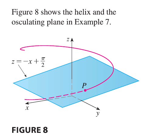
Normal Plane & Osculating Plane
The plane determined by the normal and binormal vectors \(\mathbf{N}\) and \(\mathbf{B}\) at a point P on a curve C is called the normal plane of C at P. It consists of all lines that are orthogonal to the tangent vector \(\mathbf{T}\). The plane determined by the vectors \(\mathbf{T}\) and \(\mathbf{N}\) is called the osculating plane of C at P. The name comes from the Latin osculum, meaning “kiss.” It is the plane that comes closest to containing the part of the curve near P. (For a plane curve, the osculating plane is simply the plane that contains the curve.)
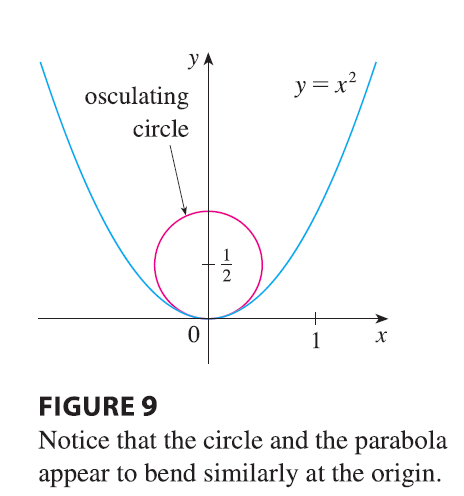
The circle that lies in the osculating plane of C at P, has the same tangent as C at P, lies on the concave side of C (toward which \(\mathbf{N}\) points), and has radius \(\rho = 1/\kappa\) (the reciprocal of the curvature) is called the osculating circle (or the circle of curvature) of C at P. It is the circle that best describes how C behaves near P; it shares the same tangent, normal, and curvature at P.
EXAMPLE 7 Find equations of the normal plane and osculating plane of the helix in Example 6 at the point \(P(0, 1, \pi/2)\).
EXAMPLE 8 Find and graph the osculating circle of the parabola \(y=x^2\) at the origin.
Section Summary
We summarize here the formulas for unit tangent, unit normal and binormal vectors, and curvature. \[ \mathbf{T}(t) = \frac{\mathbf{r}'(t)}{|\mathbf{r}'(t)|} \qquad \mathbf{N}(t) = \frac{\mathbf{T}'(t)}{|\mathbf{T}'(t)|} \qquad \mathbf{B}(t) = \mathbf{T}(t) \times \mathbf{N}(t) \] \[ \kappa = \left| \frac{d\mathbf{T}}{ds} \right| = \frac{|\mathbf{T}'(t)|}{|\mathbf{r}'(t)|} = \frac{|\mathbf{r}'(t) \times \mathbf{r}''(t)|}{|\mathbf{r}'(t)|^3} \]
Exercise 1
Find the length of the curve. \(\mathbf{r}(t) = \langle t, 3\cos t, 3\sin t \rangle, -5 \le t \le 5\)
Exercise 2
Find the length of the curve. \(\mathbf{r}(t) = \langle 2t, t^2, \frac{1}{3}t^3 \rangle, 0 \le t \le 1\)
Exercise 3
Find the length of the curve. \(\mathbf{r}(t) = \sqrt{2}t\mathbf{i} + e^t\mathbf{j} + e^{-t}\mathbf{k}, 0 \le t \le 1\)
Exercise 4
Find the length of the curve. \(\mathbf{r}(t) = \cos t \mathbf{i} + \sin t \mathbf{j} + \ln(\cos t)\mathbf{k}, 0 \le t \le \pi/4\)
Exercise 5
Find the length of the curve. \(\mathbf{r}(t) = \mathbf{i} + t^2\mathbf{j} + t^3\mathbf{k}, 0 \le t \le 1\)
Exercise 6
Find the length of the curve. \(\mathbf{r}(t) = t^2\mathbf{i} + 9t\mathbf{j} + 4t^{3/2}\mathbf{k}, 1 \le t \le 4\)
Exercise 7
Find the length of the curve correct to four decimal places. (Use a calculator to approximate the integral.) \(\mathbf{r}(t) = \langle t^2, t^3, t^4 \rangle, 0 \le t \le 2\)
Exercise 8
Find the length of the curve correct to four decimal places. (Use a calculator to approximate the integral.) \(\mathbf{r}(t) = \langle t, e^{-t}, te^{-t} \rangle, 1 \le t \le 3\)
Exercise 9
Find the length of the curve correct to four decimal places. (Use a calculator to approximate the integral.) \(\mathbf{r}(t) = \langle \cos \pi t, 2t, \sin 2\pi t \rangle\), from \((1, 0, 0)\) to \((1, 4, 0)\)
Exercise 10
Graph the curve with parametric equations \(x = \sin t, y = \sin 2t, z = \sin 3t\). Find the total length of this curve correct to four decimal places.
Exercise 11
Let C be the curve of intersection of the parabolic cylinder \(x^2=2y\) and the surface \(3z=xy\). Find the exact length of C from the origin to the point \((6, 18, 36)\).
Exercise 12
Find, correct to four decimal places, the length of the curve of intersection of the cylinder \(4x^2+y^2=4\) and the plane \(x+y+z=2\).
Exercise 13
- Find the arc length function for the curve measured from the point P in the direction of increasing t and then reparametrize the curve with respect to arc length starting from P, and (b) find the point 4 units along the curve (in the direction of increasing t) from P. \(\mathbf{r}(t) = (5-t)\mathbf{i} + (4t-3)\mathbf{j} + 3t\mathbf{k}, P(4, 1, 3)\)
Exercise 14
- Find the arc length function for the curve measured from the point P in the direction of increasing t and then reparametrize the curve with respect to arc length starting from P, and (b) find the point 4 units along the curve (in the direction of increasing t) from P. \(\mathbf{r}(t) = e^t\sin t \mathbf{i} + e^t\cos t \mathbf{j} + \sqrt{2}e^t\mathbf{k}, P(0, 1, \sqrt{2})\)
Exercise 15
Suppose you start at the point \((0, 0, 3)\) and move 5 units along the curve \(x = 3\sin t, y = 4t, z = 3\cos t\) in the positive direction. Where are you now?
Exercise 16
Reparametrize the curve \[ \mathbf{r}(t) = \left( \frac{2}{t^2+1} - 1 \right)\mathbf{i} + \frac{2t}{t^2+1}\mathbf{j} \] with respect to arc length measured from the point \((1, 0)\) in the direction of increasing t. Express the reparametrization in its simplest form. What can you conclude about the curve?
Exercise 17
- Find the unit tangent and unit normal vectors \(\mathbf{T}(t)\) and \(\mathbf{N}(t)\).
- Use Formula 9 to find the curvature. \(\mathbf{r}(t) = \langle t, 3\cos t, 3\sin t \rangle\)
Exercise 18
- Find the unit tangent and unit normal vectors \(\mathbf{T}(t)\) and \(\mathbf{N}(t)\).
- Use Formula 9 to find the curvature. \(\mathbf{r}(t) = \langle t^2, \sin t - t\cos t, \cos t + t\sin t \rangle, t > 0\)
Exercise 19
- Find the unit tangent and unit normal vectors \(\mathbf{T}(t)\) and \(\mathbf{N}(t)\).
- Use Formula 9 to find the curvature. \(\mathbf{r}(t) = \langle \sqrt{2}t, e^t, e^{-t} \rangle\)
Exercise 20
- Find the unit tangent and unit normal vectors \(\mathbf{T}(t)\) and \(\mathbf{N}(t)\).
- Use Formula 9 to find the curvature. \(\mathbf{r}(t) = \langle t, \frac{1}{2}t^2, t^2 \rangle\)
Exercise 21
Use Theorem 10 to find the curvature. \(\mathbf{r}(t) = t^3\mathbf{j} + t^2\mathbf{k}\)
Exercise 22
Use Theorem 10 to find the curvature. \(\mathbf{r}(t) = t\mathbf{i} + t^2\mathbf{j} + e^t\mathbf{k}\)
Exercise 23
Use Theorem 10 to find the curvature. \(\mathbf{r}(t) = \sqrt{6}t^2\mathbf{i} + 2t\mathbf{j} + 2t^3\mathbf{k}\)
Exercise 24
Find the curvature of \(\mathbf{r}(t) = \langle t^2, \ln t, t\ln t \rangle\) at the point \((1, 0, 0)\).
Exercise 25
Find the curvature of \(\mathbf{r}(t) = \langle t, t^2, t^3 \rangle\) at the point \((1, 1, 1)\).
Exercise 26
Graph the curve with parametric equations \(x = \cos t, y = \sin t, z = \sin 5t\) and find the curvature at the point \((1, 0, 0)\).
Exercise 27
Use Formula 11 to find the curvature. \(y = x^4\)
Exercise 28
Use Formula 11 to find the curvature. \(y = \tan x\)
Exercise 29
Use Formula 11 to find the curvature. \(y = xe^x\)
Exercise 30
At what point does the curve have maximum curvature? What happens to the curvature as \(x \to \infty\)? \(y = \ln x\)
Exercise 31
At what point does the curve have maximum curvature? What happens to the curvature as \(x \to \infty\)? \(y = e^x\)
Exercise 32
Find an equation of a parabola that has curvature 4 at the origin.
Exercise 33
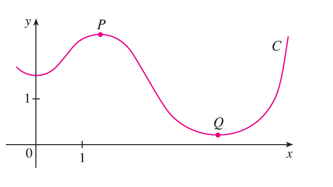
- Is the curvature of the curve C shown in the figure greater at P or at Q? Explain.
- Estimate the curvature at P and at Q by sketching the osculating circles at those points.
Exercise 34
Use a graphing calculator or computer to graph both the curve and its curvature function \(\kappa(x)\) on the same screen. Is the graph of \(\kappa\) what you would expect? \(y = x^4 - 2x^2\)
Exercise 35
Use a graphing calculator or computer to graph both the curve and its curvature function \(\kappa(x)\) on the same screen. Is the graph of \(\kappa\) what you would expect? \(y = x^{-2}\)
Exercise 36
Plot the space curve and its curvature function \(\kappa(t)\). Comment on how the curvature reflects the shape of the curve. \(\mathbf{r}(t) = \langle t - \sin t, 1 - \cos t, 4\cos(t/2) \rangle, 0 \le t \le 8\pi\)
Exercise 37
Plot the space curve and its curvature function \(\kappa(t)\). Comment on how the curvature reflects the shape of the curve. \(\mathbf{r}(t) = \langle te^t, e^{-t}, \sqrt{2}t \rangle, -5 \le t \le 5\)
Exercise 38
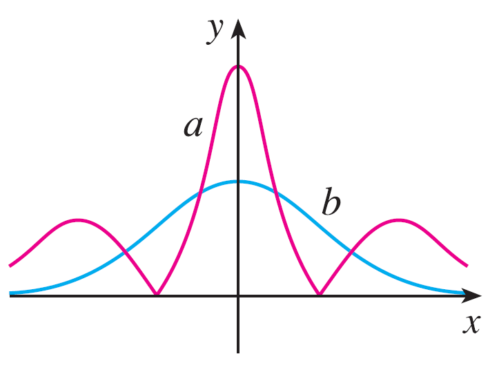
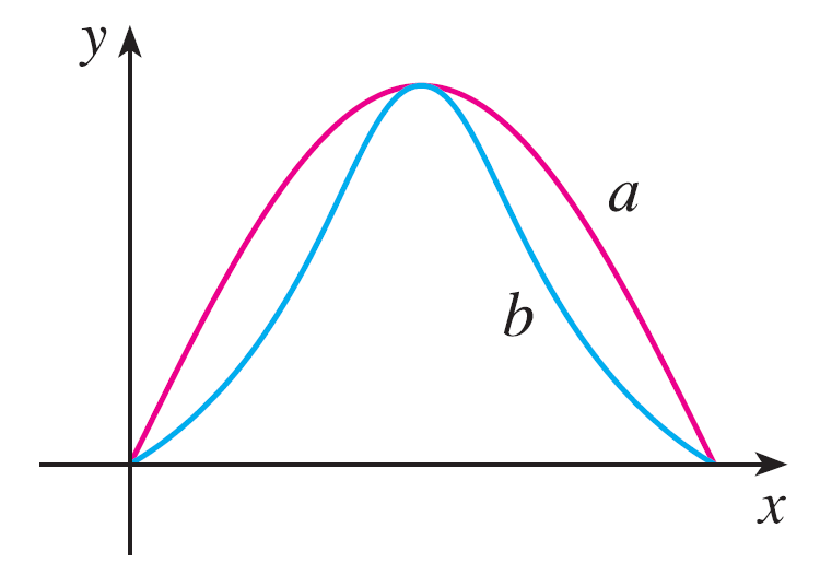
Two graphs, a and b, are shown. One is a curve \(y = f(x)\) and the other is the graph of its curvature function \(y = \kappa(x)\). Identify each curve and explain your choices.
Exercise 39
Two graphs, a and b, are shown. One is a curve \(y = f(x)\) and the other is the graph of its curvature function \(y = \kappa(x)\). Identify each curve and explain your choices.
Exercise 40
- Graph the curve \(\mathbf{r}(t) = \langle \sin 3t, \sin 2t, \sin 3t \rangle\). At how many points on the curve does it appear that the curvature has a local or absolute maximum?
- Use a CAS to find and graph the curvature function. Does this graph confirm your conclusion from part (a)?
Exercise 41
The graph of \(\mathbf{r}(t) = \langle t - \frac{3}{2}\sin t, 1 - \frac{3}{2}\cos t, t \rangle\) is shown in Figure 13.1.12(b). Where do you think the curvature is largest? Use a CAS to find and graph the curvature function. For which values of t is the curvature largest?
Exercise 42
Use Theorem 10 to show that the curvature of a plane parametric curve \(x = f(t), y = g(t)\) is \[ \kappa = \frac{|\dot{x}\ddot{y} - \dot{y}\ddot{x}|}{[\dot{x}^2 + \dot{y}^2]^{3/2}} \] where the dots indicate derivatives with respect to t.
Exercise 43
Use the formula in Exercise 42 to find the curvature. \(x = t^2, y = t^3\)
Exercise 44
Use the formula in Exercise 42 to find the curvature. \(x = a\cos \omega t, y = b\sin \omega t\)
Exercise 45
Use the formula in Exercise 42 to find the curvature. \(x = e^t\cos t, y = e^t\sin t\)
Exercise 46
Consider the curvature at \(x=0\) for each member of the family of functions \(f(x) = e^{cx}\). For which members is \(\kappa(0)\) largest?
Exercise 47
Find the vectors \(\mathbf{T}\), \(\mathbf{N}\), and \(\mathbf{B}\) at the given point. \(\mathbf{r}(t) = \langle t^2, \frac{2}{3}t^3, t \rangle, (1, \frac{2}{3}, 1)\)
Exercise 48
Find the vectors \(\mathbf{T}\), \(\mathbf{N}\), and \(\mathbf{B}\) at the given point. \(\mathbf{r}(t) = \langle \cos t, \sin t, \ln(\cos t) \rangle, (1, 0, 0)\)
Exercise 49
Find equations of the normal plane and osculating plane of the curve at the given point. \(x = \sin 2t, y = -\cos 2t, z = 4t; (0, 1, 2\pi)\)
Exercise 50
Find equations of the normal plane and osculating plane of the curve at the given point. \(x = \ln t, y = 2t, z = t^2; (0, 2, 1)\)
Exercise 51
Find equations of the osculating circles of the ellipse \(9x^2+4y^2=36\) at the points \((2, 0)\) and \((0, 3)\). Use a graphing calculator or computer to graph the ellipse and both osculating circles on the same screen.
Exercise 52
Find equations of the osculating circles of the parabola \(y = \frac{1}{2}x^2\) at the points \((0, 0)\) and \((1, \frac{1}{2})\). Graph both osculating circles and the parabola on the same screen.
Exercise 53
At what point on the curve \(x=t^3, y=3t, z=t^4\) is the normal plane parallel to the plane \(6x+6y-8z=1\)?
Exercise 54
Is there a point on the curve in Exercise 53 where the osculating plane is parallel to the plane \(x+y+z=1\)? [Note: You will need a CAS for differentiating, for simplifying, and for computing a cross product.]
Exercise 55
Find equations of the normal and osculating planes of the curve of intersection of the parabolic cylinders \(x=y^2\) and \(z=x^2\) at the point \((1, 1, 1)\).
Exercise 56
Show that the osculating plane at every point on the curve \(\mathbf{r}(t) = \langle t+2, 1-t, \frac{1}{2}t^2 \rangle\) is the same plane. What can you conclude about the curve?
Exercise 57
Show that at every point on the curve \[ \mathbf{r}(t) = \langle e^t\cos t, e^t\sin t, e^t \rangle \] the angle between the unit tangent vector and the z-axis is the same. Then show that the same result holds true for the unit normal and binormal vectors.
Exercise 58
The rectifying plane of a curve at a point is the plane that contains the vectors T and B at that point. Find the rectifying plane of the curve \(\mathbf{r}(t) = \sin t \mathbf{i} + \cos t \mathbf{j} + \tan t \mathbf{k}\) at the point \((\sqrt{2}/2, \sqrt{2}/2, 1)\).
Exercise 59
Show that the curvature \(\kappa\) is related to the tangent and normal vectors by the equation \[ \frac{d\mathbf{T}}{ds} = \kappa\mathbf{N} \]
Exercise 60
Show that the curvature of a plane curve is \(\kappa = |d\phi/ds|\), where \(\phi\) is the angle between \(\mathbf{T}\) and \(\mathbf{i}\); that is, \(\phi\) is the angle of inclination of the tangent line. (This shows that the definition of curvature is consistent with the definition for plane curves given in Exercise 10.2.69.)