Section 15.9: Change of Variables in Multiple Integrals
| Site: | Freebirds Moodle |
| Course: | Mathematical Methods I - SNIOE - Monsoon 2025 |
| Book: | Section 15.9: Change of Variables in Multiple Integrals |
| Printed by: | Guest user |
| Date: | Monday, 9 February 2026, 8:11 AM |
Table of contents
- Change of Variables in Multiple Integrals
- Shape transformation map
- Jacobian
- Change of Variables in Triple Integrals
- Exercise 1
- Exercise 2
- Exercise 3
- Exercise 4
- Exercise 5
- Exercise 6
- Exercise 7
- Exercise 8
- Exercise 9
- Exercise 10
- Exercise 11
- Exercise 12
- Exercise 13
- Exercise 14
- Exercise 15
- Exercise 16
- Exercise 17
- Exercise 18
- Exercise 19
- Exercise 20
- Exercise 21
- Exercise 22
- Exercise 23
- Exercise 24
- Exercise 25
- Exercise 26
- Exercise 27
- Exercise 28
Change of Variables in Multiple Integrals
In one-dimensional calculus we often use a change of variable (a substitution) to simplify an integral. By reversing the roles of x and u, we can write the Substitution Rule (5.5.6) as
\[ \int_a^b f(x) dx = \int_c^d f(g(u)) g'(u) du \tag{1} \]
where \(x = g(u)\) and \(a = g(c)\), \(b = g(d)\). Another way of writing Formula 1 is as follows:
\[ \int_a^b f(x) dx = \int_c^d f(x(u)) \frac{dx}{du} du \tag{2} \]
A change of variables can also be useful in double integrals. We have already seen one example of this: conversion to polar coordinates. The new variables r and \(\theta\) are related to the old variables x and y by the equations \[ x = r \cos \theta \qquad y = r \sin \theta \] and the change of variables formula (15.3.2) can be written as \[ \iint_R f(x, y) dA = \iint_S f(r\cos\theta, r\sin\theta) r dr d\theta \] where S is the region in the \(r\theta\)-plane that corresponds to the region R in the xy-plane.
Shape transformation map
More generally, we consider a change of variables that is given by a transformation T from the uv-plane to the xy-plane: \[ T(u, v) = (x, y) \] where x and y are related to u and v by the equations
\[ x = g(u, v) \qquad y = h(u, v) \tag{3} \]
or, as we sometimes write, \[ x = x(u, v) \qquad y = y(u, v) \] We usually assume that T is a \(C^1\) transformation, which means that g and h have continuous first-order partial derivatives.
A transformation T is really just a function whose domain and range are both subsets of \(\mathbb{R}^2\). If \(T(u_1, v_1) = (x_1, y_1)\), then the point \((x_1, y_1)\) is called the image of the point \((u_1, v_1)\). If no two points have the same image, T is called one-to-one.
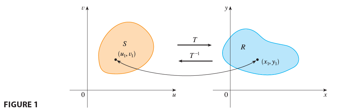
Figure 1 shows the effect of a transformation T on a region S in the uv-plane. T transforms S into a region R in the xy-plane called the image of S, consisting of the images of all points in S.
If T is a one-to-one transformation, then it has an inverse transformation \(T^{-1}\) from the xy-plane to the uv-plane and it may be possible to solve Equations 3 for u and v in terms of x and y: \[ u = G(x, y) \qquad v = H(x, y) \]
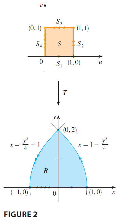
EXAMPLE 1 A transformation is defined by the equations \[ x = u^2 - v^2 \qquad y = 2uv \] Find the image of the square \(S = \{(u, v) | 0 \le u \le 1, 0 \le v \le 1\}\).
Jacobian
Now let’s see how a change of variables affects a double integral. We start with a small rectangle S in the uv-plane whose lower left corner is the point \((u_0, v_0)\) and whose dimensions are \(\Delta u\) and \(\Delta v\). (See Figure 3.)
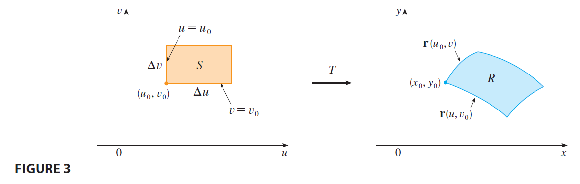
The image of S is a region R in the xy-plane, one of whose boundary points is \((x_0, y_0) = T(u_0, v_0)\). The vector \[ \mathbf{r}(u, v) = g(u, v)\mathbf{i} + h(u, v)\mathbf{j} \] is the position vector of the image of the point \((u, v)\). The equation of the lower side of S is \(v=v_0\), whose image curve is given by the vector function \(\mathbf{r}(u, v_0)\). The tangent vector at \((x_0, y_0)\) to this image curve is \[ \mathbf{r}_u = g_u(u_0, v_0)\mathbf{i} + h_u(u_0, v_0)\mathbf{j} = \frac{\partial x}{\partial u}\mathbf{i} + \frac{\partial y}{\partial u}\mathbf{j} \] Similarly, the tangent vector at \((x_0, y_0)\) to the image curve of the left side of S (namely, \(u=u_0\)) is \[ \mathbf{r}_v = g_v(u_0, v_0)\mathbf{i} + h_v(u_0, v_0)\mathbf{j} = \frac{\partial x}{\partial v}\mathbf{i} + \frac{\partial y}{\partial v}\mathbf{j} \] We can approximate the image region \(R = T(S)\) by a parallelogram determined by the secant vectors \[ \mathbf{a} = \mathbf{r}(u_0+\Delta u, v_0) - \mathbf{r}(u_0, v_0) \qquad \mathbf{b} = \mathbf{r}(u_0, v_0+\Delta v) - \mathbf{r}(u_0, v_0) \] shown in Figure 4. But
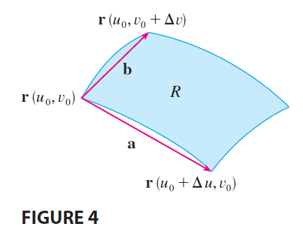
\[ \mathbf{r}_u = \lim_{\Delta u \to 0} \frac{\mathbf{r}(u_0+\Delta u, v_0) - \mathbf{r}(u_0, v_0)}{\Delta u} \] and so \[ \mathbf{r}(u_0+\Delta u, v_0) - \mathbf{r}(u_0, v_0) \approx \Delta u \mathbf{r}_u \] Similarly \[ \mathbf{r}(u_0, v_0+\Delta v) - \mathbf{r}(u_0, v_0) \approx \Delta v \mathbf{r}_v \] This means that we can approximate R by a parallelogram determined by the vectors \(\Delta u \mathbf{r}_u\) and \(\Delta v \mathbf{r}_v\). (See Figure 5.)
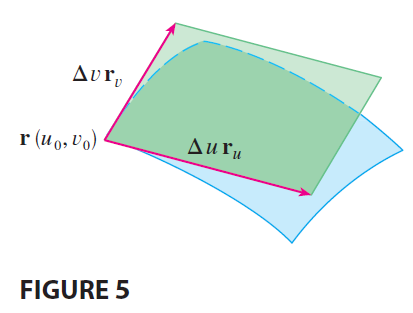
Therefore we can approximate the area of R by the area of this parallelogram, which, from Section 12.4, is
\[ |(\Delta u \mathbf{r}_u) \times (\Delta v \mathbf{r}_v)| = |\mathbf{r}_u \times \mathbf{r}_v| \Delta u \Delta v \tag{6} \]
Computing the cross product, we obtain \[ \mathbf{r}_u \times \mathbf{r}_v = \begin{vmatrix} \mathbf{i} & \mathbf{j} & \mathbf{k} \\ \frac{\partial x}{\partial u} & \frac{\partial y}{\partial u} & 0 \\ \frac{\partial x}{\partial v} & \frac{\partial y}{\partial v} & 0 \end{vmatrix} = \begin{vmatrix} \frac{\partial x}{\partial u} & \frac{\partial y}{\partial u} \\ \frac{\partial x}{\partial v} & \frac{\partial y}{\partial v} \end{vmatrix} \mathbf{k} = \left( \frac{\partial x}{\partial u}\frac{\partial y}{\partial v} - \frac{\partial y}{\partial u}\frac{\partial x}{\partial v} \right) \mathbf{k} \] The determinant that arises in this calculation is called the Jacobian of the transformation and is given a special notation.
Definition 7 The Jacobian of the transformation T given by \(x=g(u, v)\) and \(y=h(u, v)\) is \[ \frac{\partial(x, y)}{\partial(u, v)} = \begin{vmatrix} \frac{\partial x}{\partial u} & \frac{\partial x}{\partial v} \\ \frac{\partial y}{\partial u} & \frac{\partial y}{\partial v} \end{vmatrix} = \frac{\partial x}{\partial u}\frac{\partial y}{\partial v} - \frac{\partial x}{\partial v}\frac{\partial y}{\partial u} \]
With this notation we can use Equation 6 to give an approximation to the area \(\Delta A\) of R:
\[ \Delta A \approx \left| \frac{\partial(x, y)}{\partial(u, v)} \right| \Delta u \Delta v \tag{8} \]
where the Jacobian is evaluated at \((u_0, v_0)\).
Next we divide a region S in the uv-plane into rectangles \(S_{ij}\) and call their images in the xy-plane \(R_{ij}\). (See Figure 6.)
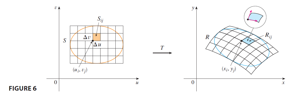
Applying the approximation (8) to each \(R_{ij}\), we approximate the double integral of f over R as follows: \[ \iint_R f(x, y) dA \approx \sum_{i=1}^m \sum_{j=1}^n f(x_i, y_j) \Delta A_{ij} \] \[ \approx \sum_{i=1}^m \sum_{j=1}^n f(g(u_i, v_j), h(u_i, v_j)) \left| \frac{\partial(x, y)}{\partial(u, v)} \right| \Delta u \Delta v \] where the Jacobian is evaluated at \((u_i, v_j)\). Notice that this double sum is a Riemann sum for the integral \[ \iint_S f(g(u, v), h(u, v)) \left| \frac{\partial(x, y)}{\partial(u, v)} \right| du dv \] The foregoing argument suggests that the following theorem is true. (A full proof is given in books on advanced calculus.)
9 Change of Variables in a Double Integral Suppose that T is a \(C^1\) transformation whose Jacobian is nonzero and that T maps a region S in the uv-plane onto a region R in the xy-plane. Suppose that f is continuous on R and that R and S are type I or type II plane regions. Suppose also that T is one-to-one, except perhaps on the boundary of S. Then \[ \iint_R f(x, y) dA = \iint_S f(x(u, v), y(u, v)) \left| \frac{\partial(x, y)}{\partial(u, v)} \right| du dv \]
Theorem 9 says that we change from an integral in x and y to an integral in u and v by expressing x and y in terms of u and v and writing \[ dA = \left| \frac{\partial(x, y)}{\partial(u, v)} \right| du dv \] Notice the similarity between Theorem 9 and the one-dimensional formula in Equation 2. Instead of the derivative \(dx/du\), we have the absolute value of the Jacobian, that is, \(|\partial(x, y)/\partial(u, v)|\).
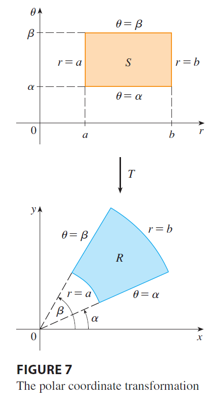
As a first illustration of Theorem 9, we show that the formula for integration in polar coordinates is just a special case. Here the transformation T from the \(r\theta\)-plane to the xy-plane is given by \[ x = g(r, \theta) = r\cos\theta \qquad y = h(r, \theta) = r\sin\theta \] and the geometry of the transformation is shown in Figure 7. T maps an ordinary rectangle in the \(r\theta\)-plane to a polar rectangle in the xy-plane. The Jacobian of T is \[ \frac{\partial(x, y)}{\partial(r, \theta)} = \begin{vmatrix} \frac{\partial x}{\partial r} & \frac{\partial x}{\partial \theta} \\ \frac{\partial y}{\partial r} & \frac{\partial y}{\partial \theta} \end{vmatrix} = \begin{vmatrix} \cos\theta & -r\sin\theta \\ \sin\theta & r\cos\theta \end{vmatrix} = r\cos^2\theta + r\sin^2\theta = r > 0 \]
Thus Theorem 9 gives \[ \iint_R f(x, y) dx dy = \iint_S f(r\cos\theta, r\sin\theta) \left| \frac{\partial(x, y)}{\partial(r, \theta)} \right| dr d\theta \] \[ = \int_\alpha^\beta \int_a^b f(r\cos\theta, r\sin\theta) r dr d\theta \] which is the same as Formula 15.3.2.
EXAMPLE 2 Use the change of variables \(x = u^2 - v^2, y = 2uv\) to evaluate the integral \(\iint_R y dA\), where R is the region bounded by the x-axis and the parabolas \(y^2 = 4-4x\) and \(y^2 = 4+4x, y \ge 0\).
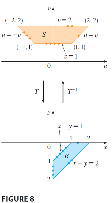
EXAMPLE 3 Evaluate the integral \(\iint_R e^{(x+y)/(x-y)} dA\), where R is the trapezoidal region with vertices \((1, 0), (2, 0), (0, -2),\) and \((0, -1)\).
Change of Variables in Triple Integrals
There is a similar change of variables formula for triple integrals. Let T be a transformation that maps a region S in uvw-space onto a region R in xyz-space by means of the equations \[ x = g(u, v, w) \qquad y = h(u, v, w) \qquad z = k(u, v, w) \] The Jacobian of T is the following \(3 \times 3\) determinant:
\[ \frac{\partial(x, y, z)}{\partial(u, v, w)} = \begin{vmatrix} \frac{\partial x}{\partial u} & \frac{\partial x}{\partial v} & \frac{\partial x}{\partial w} \\ \frac{\partial y}{\partial u} & \frac{\partial y}{\partial v} & \frac{\partial y}{\partial w} \\ \frac{\partial z}{\partial u} & \frac{\partial z}{\partial v} & \frac{\partial z}{\partial w} \end{vmatrix} \tag{12} \]
Under hypotheses similar to those in Theorem 9, we have the following formula for triple integrals:
\[ \iiint_R f(x, y, z) dV = \iiint_S f(x(u,v,w), y(u,v,w), z(u,v,w)) \left| \frac{\partial(x,y,z)}{\partial(u,v,w)} \right| du dv dw \tag{13} \]
EXAMPLE 4 Use Formula 13 to derive the formula for triple integration in spherical coordinates.
Exercise 1
Find the Jacobian of the transformation. \(x = 2u+v, y = 4u-v\)
Exercise 2
Find the Jacobian of the transformation. \(x = u^2+uv, y = uv^2\)
Exercise 3
Find the Jacobian of the transformation. \(x = s\cos t, y = s\sin t\)
Exercise 4
Find the Jacobian of the transformation. \(x = pe^q, y = qe^p\)
Exercise 5
Find the Jacobian of the transformation. \(x = uv, y = vw, z = wu\)
Exercise 6
Find the Jacobian of the transformation. \(x = u+vw, y = v+wu, z = w+uv\)
Exercise 7
Find the image of the set S under the given transformation. \(S = \{(u, v) | 0 \le u \le 3, 0 \le v \le 2\}; x = 2u+3v, y = u-v\)
Exercise 8
Find the image of the set S under the given transformation. S is the square bounded by the lines \(u=0, u=1, v=0, v=1; x=v, y=u(1+v^2)\)
Exercise 9
Find the image of the set S under the given transformation. S is the triangular region with vertices \((0, 0), (1, 1), (0, 1); x=u^2, y=v\)
Exercise 10
Find the image of the set S under the given transformation. S is the disk given by \(u^2+v^2 \le 1; x=au, y=bv\)
Exercise 11
A region R in the xy-plane is given. Find equations for a transformation T that maps a rectangular region S in the uv-plane onto R, where the sides of S are parallel to the u- and v-axes. R is bounded by \(y=2x-1, y=2x+1, y=1-x, y=3-x\)
Exercise 12
A region R in the xy-plane is given. Find equations for a transformation T that maps a rectangular region S in the uv-plane onto R, where the sides of S are parallel to the u- and v-axes. R is the parallelogram with vertices \((0, 0), (4, 3), (2, 4), (-2, 1)\)
Exercise 13
A region R in the xy-plane is given. Find equations for a transformation T that maps a rectangular region S in the uv-plane onto R, where the sides of S are parallel to the u- and v-axes. R lies between the circles \(x^2+y^2=1\) and \(x^2+y^2=2\) in the first quadrant.
Exercise 14
A region R in the xy-plane is given. Find equations for a transformation T that maps a rectangular region S in the uv-plane onto R, where the sides of S are parallel to the u- and v-axes. R is bounded by the hyperbolas \(y=1/x, y=4/x\) and the lines \(y=x, y=4x\) in the first quadrant.
Exercise 15
Use the given transformation to evaluate the integral. \(\iint_R (x-3y) dA\), where R is the triangular region with vertices \((0, 0), (2, 1),\) and \((1, 2); x=2u+v, y=u+2v\)
Exercise 16
Use the given transformation to evaluate the integral. \(\iint_R (4x+8y) dA\), where R is the parallelogram with vertices \((-1, 3), (1, -3), (3, -1),\) and \((1, 5); x=\frac{1}{4}(u+v), y=\frac{1}{4}(v-3u)\)
Exercise 17
Use the given transformation to evaluate the integral. \(\iint_R x^2 dA\), where R is the region bounded by the ellipse \(9x^2+4y^2=36; x=2u, y=3v\)
Exercise 18
Use the given transformation to evaluate the integral. \(\iint_R (x^2-xy+y^2) dA\), where R is the region bounded by the ellipse \(x^2-xy+y^2=2; x=\sqrt{2}u - \sqrt{2/3}v, y=\sqrt{2}u + \sqrt{2/3}v\)
Exercise 19
Use the given transformation to evaluate the integral. \(\iint_R xy \, dA\), where R is the region in the first quadrant bounded by the lines \(y=x\) and \(y=3x\) and the hyperbolas \(xy=1, xy=3; x=u/v, y=v\)
Exercise 20
Use the given transformation to evaluate the integral. \(\iint_R y^2 \, dA\), where R is the region bounded by the curves \(xy=1, xy=2, xy^2=1, xy^2=2; u=xy, v=xy^2\). Illustrate by using a graphing calculator or computer to draw R.
Exercise 21
- Evaluate \(\iiint_E dV\), where E is the solid enclosed by the ellipsoid \(\frac{x^2}{a^2} + \frac{y^2}{b^2} + \frac{z^2}{c^2} = 1\). Use the transformation \(x=au, y=bv, z=cw\).
- The earth is not a perfect sphere; rotation has resulted in flattening at the poles. So the shape can be approximated by an ellipsoid with \(a=b=6378\) km and \(c=6356\) km. Use part (a) to estimate the volume of the earth.
- If the solid of part (a) has constant density k, find its moment of inertia about the z-axis.
Exercise 22
An important problem in thermodynamics is to find the work done by an ideal Carnot engine. A cycle consists of alternating expansion and compression of gas in a piston. The work done by the engine is equal to the area of the region R enclosed by two isothermal curves \(xy=a, xy=b\) and two adiabatic curves \(xy^{1.4}=c, xy^{1.4}=d\), where \(0 < a < b\) and \(0 < c < d\). Compute the work done by determining the area of R.
Exercise 23
Evaluate the integral by making an appropriate change of variables. \(\iint_R \frac{x-2y}{3x-y} dA\), where R is the parallelogram enclosed by the lines \(x-2y=0, x-2y=4, 3x-y=1,\) and \(3x-y=8\).
Exercise 24
Evaluate the integral by making an appropriate change of variables. \(\iint_R (x+y)e^{x^2-y^2} dA\), where R is the rectangle enclosed by the lines \(x-y=0, x-y=2, x+y=0,\) and \(x+y=3\).
Exercise 25
Evaluate the integral by making an appropriate change of variables. \(\iint_R \cos\left(\frac{y-x}{y+x}\right) dA\), where R is the trapezoidal region with vertices \((1, 0), (2, 0), (0, 2),\) and \((0, 1)\).
Exercise 26
Evaluate the integral by making an appropriate change of variables. \(\iint_R \sin(9x^2+4y^2) dA\), where R is the region in the first quadrant bounded by the ellipse \(9x^2+4y^2=1\).
Exercise 27
Evaluate the integral by making an appropriate change of variables. \(\iint_R e^{x+y} dA\), where R is given by the inequality \(|x|+|y| \le 1\).
Exercise 28
Let f be continuous on \([0, 1]\) and let R be the triangular region with vertices \((0, 0), (1, 0),\) and \((0, 1)\). Show that \[ \iint_R f(x+y) dA = \int_0^1 u f(u) du \]