Space curves are inherently more difficult to draw by hand than plane
curves; for an accurate representation we need to use technology. For
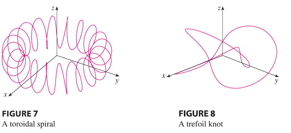
instance, Figure 7 shows a computer-generated graph of the curve with
parametric equations \[ x = (4 + \sin
20t)\cos t \qquad y = (4 + \sin 20t)\sin t \qquad z = \cos 20t
\]
It’s called a toroidal spiral because it lies on a
torus. Another interesting curve, the trefoil knot,
with equations \[ x = (2 + \cos 1.5t)\cos t
\qquad y = (2 + \cos 1.5t)\sin t \qquad z = \sin 1.5t \] is
graphed in Figure 8. It wouldn’t be easy to plot either of these curves
by hand.
Even when a computer is used to draw a space curve, optical illusions
make it difficult to get a good impression of what the curve really
looks like. (This is especially true in Figure 8. See Exercise 52.) The
next example shows how to cope with this problem.
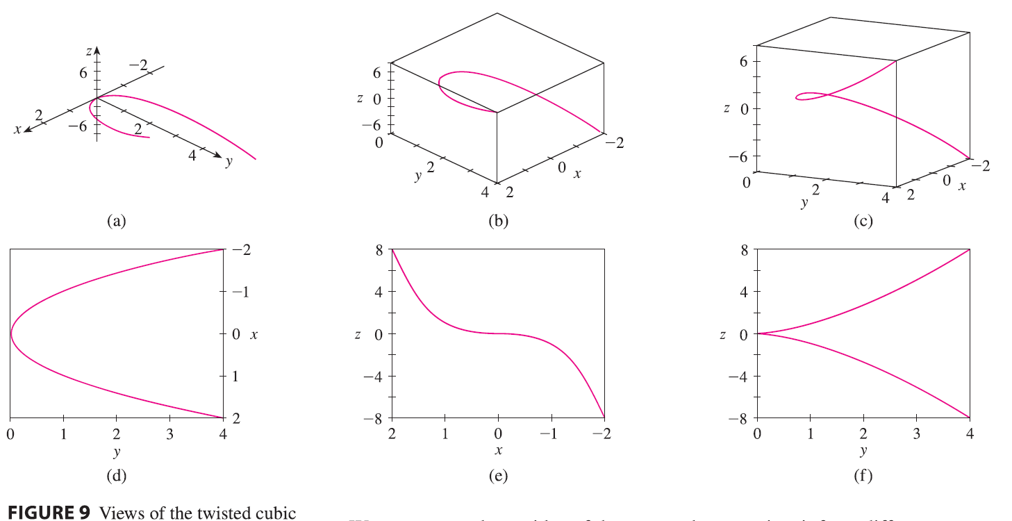
EXAMPLE 7 Use a computer to draw the curve with
vector equation \(\mathbf{r}(t) = \langle t,
t^2, t^3 \rangle\). This curve is called a twisted
cubic.
SOLUTION We start by using the computer to plot the
curve with parametric equations \(x=t, y=t^2,
z=t^3\) for \(-2 \le t \le 2\).
The result is shown in Figure 9(a), but it’s hard to see the true nature
of the curve from that graph alone. Most three-dimensional computer
graphing programs allow the user to enclose a curve or surface in a box
instead of displaying the coordinate axes. When we look at the same
curve in a box in Figure 9(b), we have a much clearer picture of the
curve. We can see that it climbs from a lower corner of the box to the
upper corner nearest us, and it twists as it climbs.
We get an even better idea of the curve when we view it from
different vantage points. Part (c) shows the result of rotating the box
to give another viewpoint. Parts (d), (e), and (f) show the views we get
when we look directly at a face of the box. In particular, part (d)
shows the view from directly above the box. It is the projection of the
curve onto the xy-plane, namely, the parabola \(y=x^2\). Part (e) shows the projection onto
the xz-plane, the cubic curve \(z=x^3\). It’s now obvious why the given
curve is called a twisted cubic.
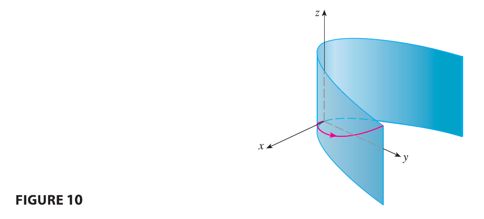
Another method of visualizing a space curve is to draw it on a
surface. For instance, the twisted cubic in Example 7 lies on the
parabolic cylinder \(y=x^2\).
(Eliminate the parameter from the first two parametric equations, \(x=t\) and \(y=t^2\).) Figure 10 shows both the cylinder
and the twisted cubic, and we see that the curve moves upward from the
origin along the surface of the cylinder.
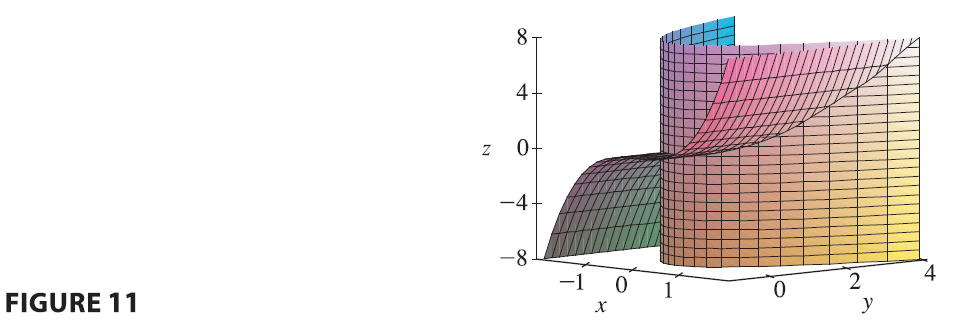
A third method for visualizing the twisted cubic is to realize that
it also lies on the cylinder \(z=x^3\).
So it can be viewed as the curve of intersection of the cylinders \(y=x^2\) and \(z=x^3\). (See Figure 11.)